Recursion
Source: this section is heavily based on Chapter 18 of [ThinkCS].
Recursion means "defining something in terms of itself" usually at some smaller scale, perhaps multiple times, to achieve some objective. For example, we might say "A human being is someone whose parents are human beings", or "a directory is a structure that holds files and (smaller) directories", or "a family tree starts with a couple who have children, each with their own family sub-trees".
Programming languages generally support recursion, which means that, in order to solve a problem, functions can call themselves to solve smaller subproblems.
Drawing Fractals
A fractal is a drawing that has self-similar structure, which can be defined in terms of itself. [Fractal]
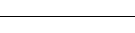
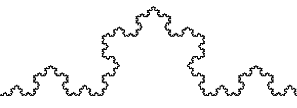
Let us start by looking at the famous Koch fractal. An order 0 Koch fractal is simply a straight line of a given size.
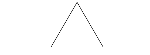
An order 1 Koch fractal is obtained like this: instead of drawing just one line, draw instead four smaller segments, as in the pattern shown below.
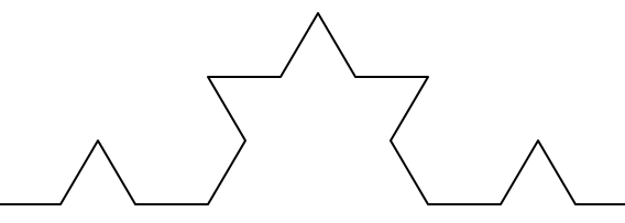
Now what would happen if we repeated this Koch pattern again on each of the order 1 segments? We'd get an order 2 Koch fractal.
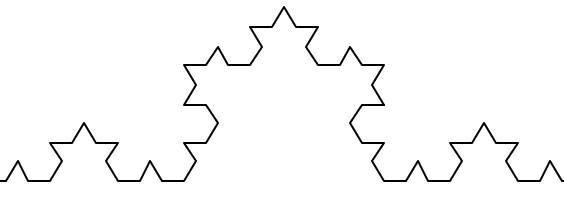
Repeating our pattern again gets us an order 3 Koch fractal.
And so on, and so forth. For example this is an order 5 Koch fractal.
Now let us think about it the other way around. To draw a Koch fractal of order 3, we can simply draw four order 2 Koch fractals. But each of these in turn needs four order 1 Koch fractals, and each of those in turn needs four order 0 fractals. Ultimately, the only drawing that will take place is at order 0. This is very simple to code up in Python:
def koch(t, order, size):
    """
       Makes turtle 't' draw a Koch fractal of 'order' and 'size'.
       pre:  't' is a Turtle object, ready to draw on some Screen
       post: A Koch fractal of given 'order' and 'size' has been
             drawn by turtle 't' on the screen, and the turtle 't'
             is left facing the same direction.
    """

    if order == 0:          # The base case is just a straight line
        t.forward(size)
    else:
        koch(t, order-1, size/3)   # Go 1/3 of the way
        t.left(60)
        koch(t, order-1, size/3)
        t.right(120)
        koch(t, order-1, size/3)
        t.left(60)
        koch(t, order-1, size/3)

"Of course, to actually run the code above we still need to"
"add the necessary instructions to set up the turtle graphics:"

import turtle
window = turtle.Screen()
t = turtle.Turtle()
t.speed(0)
t.penup()
t.forward(-150)
t.pendown()
koch(t,5,300)     # <- Here is the actual call to the koch function !
window.mainloop()
The key thing that is new here is that as long as order is not zero, koch calls itself recursively to get its job done.
Rereading the above code of the koch function, we observe that it contains a quite repetitive pattern. (Do you see it?) Not quite fond of duplicated code, we will try to tighten up the code a bit to get rid of this repetition. First of all, remember that turning right by 120 degrees is the same as turning left by -120 degrees. So with a bit of clever rearrangement, we can use a single loop to make the four recursive calls to the koch function in the else-branch.
def koch(t, order, size):
    if order == 0:
        t.forward(size)
    else:
        for angle in [60, -120, 60, 0]:
           koch(t, order-1, size/3)
           t.left(angle)
The final turn is 0 degrees, so it has no effect. But it has allowed us to find a pattern and reduce seven lines of code to three, which will make things easier for our next observations.
Recursion, the high-level view
One way to think about this is to convince yourself that the function works correctly when you call it for an order 0 fractal. Then do a mental leap of faith, saying "I will assume that Python will handle correctly the four recursive level 0 calls for me in the else-branch, so I don't need to think about that detail. So all I need to focus on now is how to draw an order 1 fractal assuming that the order 0 one is already working."
You're practicing mental abstraction --- ignoring the subproblem while you solve the big problem.
If this mode of thinking works (and you should practice it!), then take it to the next level. Aha! now can I see that it will work when called for order 2 under the assumption that it is already working for level 1.
And, in general, if I can assume the order n-1 case works, can I just solve the level n problem?
Students of mathematics who have played with proofs of induction should see some very strong similarities here.
Recursion, the low-level operational view
Another way of trying to understand recursion is to get rid of it! If we had separate functions to draw a level 3 fractal, a level 2 fractal, a level 1 fractal and a level 0 fractal, we could simplify the above code, quite mechanically, to a situation where there was no longer any recursion, like this:
def koch_0(t, size):
    t.forward(size)

def koch_1(t, size):
    for angle in [60, -120, 60, 0]:
       koch_0(t, size/3)
       t.left(angle)

def koch_2(t, size):
    for angle in [60, -120, 60, 0]:
       koch_1(t, size/3)
       t.left(angle)

def koch_3(t, size):
    for angle in [60, -120, 60, 0]:
       koch_2(t, size/3)
       t.left(angle)
This trick of "unfolding" the recursion gives us an operational view of what happens. You can trace the program into koch_3, and from there, into koch_2, and then into koch_1, etc., all the way down the different layers of the recursion.
This might be a useful hint to build your understanding. The mental goal is, however, to be able to do the abstraction!
Recursive data structures
All of the Python data types we have seen can be grouped inside lists and tuples in a variety of ways. Lists and tuples can also be nested, providing many possibilities for organizing data. The organization of data for the purpose of making it easier to use is called a data structure.
Suppose it is election time and that we are helping to count votes as they come in. Votes arriving from individual districts, cities, agglomerations and provinces are sometimes reported as a sum total of votes and sometimes as a list of subtotals of votes. After considering how best to store this incoming data, we decide to use a nested number list, which we define as follows:
A nested number list is a list whose elements are either:
- numbers
- nested number lists
Notice how in the above definition, the term nested number list is used to define itself. Recursive definitions like this are quite common in mathematics and computer science. They provide a concise and powerful way to describe recursive data structures that are partially composed of smaller and simpler instances of themselves. The definition is not circular, nor infinite, since at some point we will reach a list that does not have any lists as elements.
Now suppose our job is to write a function that will sum all of the values in a nested number list. Python has a built-in function which finds the sum of a sequence of numbers:
>>> sum([1, 2, 8])
11
For our nested number list, however, sum will not work:
>>> sum([1, 2, [11, 13], 8])
Traceback (most recent call last):
  File "<pyshell>", line 1, in <module>
TypeError: unsupported operand type(s) for +: 'int' and 'list'
The problem is that the third element of this list, [11, 13], is itself a list, so it cannot just be added to 1, 2, and 8.
Processing recursive number lists
To sum all the numbers in our recursive nested number list we need to traverse the list, visiting each of the elements within its nested structure, adding any numeric elements to our sum, and recursively repeating the summing process with any elements which are themselves sub-lists.
Thanks to recursion, the Python code needed to sum the values of a nested number list is surprisingly short:
def r_sum(nested_num_list):
    """
      Computes the sum of all values in a recursively nested structure of lists.
      pre:  'nested_num_list' is a nested number list, i.e., a list whose elements
            are either numbers or again nested number lists.
      post: returns 0 for empty lists or the sum of all encountered values,
            at any level of nesting, for nested number lists.
    """
    tot = 0
    for element in nested_num_list:
        if isinstance(element,list):
            tot += r_sum(element)
        else:
            tot += element
    return tot
>>> r_sum([1, 2, [11, 13], 8])
35
The body of r_sum consists mainly of a for loop that traverses nested_num_list. If element is a numerical value (the else branch), it is simply added to tot. If element is a list (which is checked with the type check isinstance(element,list)), then r_sum is called again, with the element as an argument. The statement inside the function definition in which the function calls itself is known as the recursive call.
The example above has a base case (the else branch) which does not lead to a recursive call: the case where the element is not a (sub-) list. Without a base case, you'll have infinite recursion, and your program will not work.
Recursion is truly one of the most beautiful and elegant tools in computer science.
A slightly more complicated problem is finding the largest value in a nested number list:
def r_max(nxs):
    """
      Finds the maximum value in a recursively nested structure of lists.
      pre:  'nxs' is a nested number list, i.e., a list whose elements
            are either numbers or again nested number lists.
            No lists or sublists are empty.
      post: returns the maximum value of all encountered values
            in this nested structure of lists.
    """
    largest = None
    first_time = True
    for e in nxs:
        if isinstance(e,list):
            val = r_max(e)
        else:
            val = e

        if first_time or val > largest:
            largest = val
            first_time = False

    return largest

test(r_max([2, 9, [1, 13], 8, 6]) == 13)
test(r_max([2, [[100, 7], 90], [1, 13], 8, 6]) == 100)
test(r_max([[[13, 7], 90], 2, [1, 100], 8, 6]) == 100)
test(r_max(["joe", ["sam", "ben"]]) == "sam")
We included some tests to provide examples of r_max at work. (All these assertions should succeed. Figure out for yourself what would happen if the list or one of its nested sublists would be empty.)
The added twist to this problem is finding a value for initializing largest. We can't just use nxs[0], since that could be either an element or a list. To solve this problem (at every recursive call) we set a Boolean flag first_time to True (at line 11). When we've found the value of interest (at line 17), we check to see whether this is the initializing (first) value for largest, or a value that could potentially change largest.
Again here we have a base case at line 15. If we don't supply a base case, Python stops after reaching a maximum recursion depth and returns a runtime error. See how this happens, by running this little script which we will call infinite_recursion.py:
def recursion_depth(number):
    print("{0}, ".format(number), end="")
    recursion_depth(number + 1)

recursion_depth(0)
After watching the messages flash by, you will be presented with the end of a long traceback that ends with a message like the following:
RecursionError: maximum recursion depth exceeded while calling a Python object
We would certainly never want something like this to happen to a user of one of our programs, so it is good programming practice to write error handling code that could handle such errors when they arise.
Fibonacci numbers
The famous Fibonacci sequence 0, 1, 1, 2, 3, 5, 8, 13, 21, 34, 55, 89, 144, ... [FibonacciNumber] was devised by Fibonacci (1170-1250), who used this to model the breeding of (pairs) of rabbits. If, in generation 8 you had 21 pairs in total, of which 13 were adults, then next generation the adults will all have bred new children, and the previous children will have grown up to become adults. So in generation 9 you'll have 13+21=34, of which 21 are adults.
This model to explain rabbit breeding made the simplifying assumption that rabbits never died. Scientists often make (over-)simplifying assumptions and restrictions to make some headway with the problem.
If we number the terms of the sequence from 0, we can describe each term recursively as the sum of the previous two terms:
fib(0) = 0
fib(1) = 1
fib(n) = fib(n-1) + fib(n-2)  for n >= 2
This translates very directly into some Python:
def fib(n):
    """
      Computes numbers in the Fibonacci sequence 0, 1, 1, 2, 3, 5, 8, 13, 21, ...
      pre:  'n' is natural number (an integer >= 0)
      post: returns the n-th Fibonacci number,
            where fib(0) = 0 and fib(1) = 1
            and any other Fibonacci number is defined
            as the sum of the previous 2 Fibonacci numbers,
            for example: fib(2) = fib(0) + fib(1) = 0 + 1 = 1
    """
    if n <= 1:
        return n
    t = fib(n-1) + fib(n-2)
    return t

test(fib(0) == 0)
test(fib(1) == 1)
test(fib(2) == 1)
test(fib(3) == 2)
test(fib(4) == 3)
test(fib(5) == 5)
test(fib(6) == 8)
test(fib(7) == 13)
test(fib(8) == 21)
test(fib(9) == 34)
test(fib(10) == 55)
test(fib(11) == 89)
test(fib(12) == 144)
This is a particularly inefficient algorithm. One particular way of fixing this inefficiency, which we will leave as an exercise for now, is to make use of dictionaries to remember (or memoize) previously calculated values of the function so that they don't need to be recalculated over and over again.
import time
from time import process_time
t0 = process_time()
n = 35
result = fib(n)
t1 = process_time()

print("fib({0}) = {1}, ({2:.2f} secs)".format(n, result, t1-t0))
We get the correct result, but an exploding amount of work!
fib(35) = 9227465, (4.51 secs)
Memoization
If you play around a bit with the fib function from the previous section, you will notice that the bigger the argument you provide, the longer the function takes to run. Furthermore, the run time increases very quickly. On one of our machines, fib(20) finishes instantly, fib(30) takes about a second, and fib(40) takes roughly forever.
To understand why, consider this call graph for fib with n = 4:
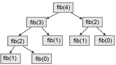
A call graph shows some function frames (instances when the function has been invoked), with lines connecting each frame to the frames of the functions it calls. At the top of the graph, fib with n = 4 calls fib with n = 3 and n = 2. In turn, fib with n = 3 calls fib with n = 2 and n = 1. And so on.
Count how many times fib(0) and fib(1) are called. This is an inefficient solution to the problem, and it gets far worse as the argument gets bigger.
A good solution is to keep track of values that have already been computed by storing them in a dictionary. A previously computed value that is stored for later use is called a memo. Here is an implementation of fib using memos:
alreadyknown = {0: 0, 1: 1}

def fib(n):
    if n not in alreadyknown:
        new_value = fib(n-1) + fib(n-2)
        alreadyknown[n] = new_value
    return alreadyknown[n]
The dictionary named alreadyknown keeps track of the Fibonacci numbers we already know. We start with only two pairs: 0 maps to 1; and 1 maps to 1.
Whenever fib is called, it checks the dictionary to determine if it contains the result. If it's there, the function can return immediately without making any more recursive calls. If not, it has to compute the new value. The new value is added to the dictionary before the function returns.
Using this version of fib, our machines can compute fib(100) in an eyeblink.
>>> fib(100)
354224848179261915075
Example with recursive directories and files
The following program lists the contents of a directory and all its subdirectories. Notice how a recursive function print_files is used to recursively walk through the recursively nested directory structure.
import os

def get_dirlist(path):
    """
      Produces the list of all files in a given directory.
      pre:  'path' is a string describing a valid path to a directory
            in the operating system.
      post: Returns a sorted list of the names of all entries (files
            or directories) encountered in the directory with that path.
            This returns just the names, not the full path to the names.
            Directories nested in this directory are not recursively explored.
    """
    dirlist = os.listdir(path)
    dirlist.sort()
    return dirlist

def print_files(path, prefix = ""):
    """
      Prints the recursive listing of all contents in a given directory.
      pre:  'path' is a string describing a valid path to a directory
            in the operating system.
      post: Prints the path and the names of all entries (files or directories
            contained in it). Nested directories are visited recursively.
            For every entry, the nesting level is indicated by vertical bars.
            Entries directly contained in the path are preceded by one bar,
            entries at nesting level 2 by two bars, and so on.
    """
    if prefix == "":  # Detect outermost call, print a heading
        print("Folder listing for", path)
        prefix = "| "

    dirlist = get_dirlist(path)
    for f in dirlist:
        print(prefix+f)                    # Print the line
        fullname = os.path.join(path, f)   # Turn name into full pathname
        if os.path.isdir(fullname):        # If a directory, recurse.
            print_files(fullname, prefix + "| ")
Calling the function print_files with some initial path or folder name will produce an output similar to this:
print_files("c:\python31\Lib\site-packages\pygame\examples")

Folder listing for c:\python31\Lib\site-packages\pygame\examples
| __init__.py
| aacircle.py
| aliens.py
| arraydemo.py
| blend_fill.py
| blit_blends.py
| camera.py
| chimp.py
| cursors.py
| data
| | alien1.png
| | alien2.png
| | alien3.png
...
Glossary
- base case
- A branch of the conditional statement in a recursive function that does not give rise to further recursive calls.
- infinite recursion
- A function that calls itself recursively without ever reaching any base case. Eventually, infinite recursion causes a runtime error.
- recursion
- The process of calling a function that is already executing.
- recursive call
- The statement that calls an already executing function. Recursion can also be indirect --- function f can call g which calls h, and h could make a call back to f --- or mutual --- function f calls g and g makes a call back to f.
- recursive definition
- A definition which defines something in terms of itself. To be useful it must include base cases which are not recursive. In this way it differs from a circular definition. Recursive definitions often provide an elegant way to express complex data structures, like a directory that can contain other directories, or a menu that can contain other menus.
References
| [ThinkCS] | How To Think Like a Computer Scientist --- Learning with Python 3 |
| [Fractal] | https://en.wikipedia.org/wiki/Fractal |
| [FibonacciNumber] | https://en.wikipedia.org/wiki/Fibonacci_number |
Higher-Order Functions
Source: This section is heavily based on Section 1.6 of [SICP]. It does not appear in [ThinkCS].
We have seen before that functions are abstractions that describe compound operations independent of the particular values of their arguments. For example, when defining a function square,
def square(x):
    return x * x
we are not talking about the square of a particular number, but rather about a method for obtaining the square of any number x. Of course we could get along without ever defining this function, by always writing expressions such as:
>>> 3 * 3
9
>>> 5 * 5
25
and never mentioning square explicitly. This practice would suffice for simple computations like square, but would become arduous for more complex examples. In general, lacking function definition would put us at the disadvantage of forcing us to work always at the level of the particular operations that happen to be primitives in the language (multiplication, in this case) rather than in terms of higher-level operations. Our programs would be able to compute squares, but our language would lack the ability to express the concept of squaring. One of the things we demand from a powerful programming language is the ability to build abstractions by assigning names to common patterns and then to work in terms of these abstractions directly. Functions provide this ability.
As we will see in the following examples, there are common programming patterns that recur in code, but are used with a number of different functions. These patterns can also be abstracted, by giving them names.
To express certain general patterns as named concepts, we will need to construct functions that can accept other functions as arguments or that return functions as values. Such functions that manipulate functions are called higher-order functions. This section shows how higher-order functions can serve as powerful abstraction mechanisms, vastly increasing the expressive power of our language.
Functions as Arguments
Consider the following three functions, which all compute summations. The first, sum_naturals, computes the sum of natural numbers up to n:
def sum_naturals(n):
    total, k = 0, 1
    while k <= n:
        total, k = total + k, k + 1
    return total
>>> sum_naturals(100)
5050
The second, sum_cubes, computes the sum of the cubes of natural numbers up to n.
def sum_cubes(n):
    total, k = 0, 1
    while k <= n:
        total, k = total + pow(k, 3), k + 1
    return total
>>> sum_cubes(100)
25502500
The third, pi_sum, computes the sum of terms in the series
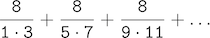
which converges to pi, though very slowly.
def pi_sum(n):
    total, k = 0, 1
    while k <= n:
        total, k = total + 8 / (k * (k + 2)), k + 4
    return total
>>> pi_sum(100)
3.121594652591009
These three functions clearly share a common underlying pattern. They are for the most part identical, differing only in their name, the function of k used to compute the term to be added, and the function that provides the next value of k. We could generate each of the functions by filling in the slots <name>, <term> and <next> in the following template:
def <name>(n):
    total, k = 0, 1
    while k <= n:
        total, k = total + <term>(k), <next>(k)
    return total
The presence of such a common pattern is strong evidence that there is a useful abstraction waiting to be brought to the surface. Each of these functions is a summation of terms. As program designers, we would like our language to be powerful enough so that we can write a function that expresses the concept of summation itself rather than only functions that compute particular sums. We can do so readily in Python by taking the common template shown above and transforming the "slots" into formal parameters of a more general summation function.
def summation(n, term, next):
    total, k = 0, 1
    while k <= n:
        total, k = total + term(k), next(k)
    return total
Notice that summation takes as its arguments the upper bound n together with the functions term and next. We can use summation just as we would any function, and it expresses summations succinctly. For example, we could rewrite our earlier definition of sum_cubes(n) by making use of summation as follows:
def cube(k):
    return pow(k, 3)

def successor(k):
    return k + 1

def sum_cubes(n):
    return summation(n, cube, successor)
>>> sum_cubes(3)
36
Using as term function an identity function that returns its argument, we can also sum integers.
def identity(k):
    return k

def sum_naturals(n):
    return summation(n, identity, successor)
>>> sum_naturals(10)
55
We can even define pi_sum piece by piece, using our summation abstraction to combine components.
def pi_term(k):
    denominator = k * (k + 2)
    return 8 / denominator

def pi_next(k):
    return k + 4

def pi_sum(n):
    return summation(n, pi_term, pi_next)
>>> pi_sum(1e6)
3.1415906535898936
Functions as General Methods of Computation
We introduced user-defined functions as a mechanism for abstracting patterns of numerical operations so as to make them independent of the particular numbers involved. With higher-order functions, we begin to see a more powerful kind of abstraction: some functions express general methods of computation, independent of the particular functions they call.
To illustrate this mechanism, in this subsection we will build an abstraction for a general method of computation known as iterative improvement, and use it to compute the golden ratio [GoldenRatio]. An iterative improvement algorithm begins with a guess of a solution to an equation. It then repeatedly applies an update function to improve that guess, and applies a test to check whether the current guess is "close enough" to the expected solution to be considered correct.
def iter_improve(update, test, guess=1):
    while not test(guess):
        guess = update(guess)
    return guess
The test function typically checks whether two functions, f and g, are near to each other for a particular value of guess. Testing whether f(x) is near to g(x) is again a general method of computation.
def near(x, f, g):
    return approx_eq(f(x), g(x))
A common way to test for approximate equality in programs is to compare the absolute value of the difference between numbers to a small tolerance value.
def approx_eq(x, y, tolerance=1e-5):
    return abs(x - y) < tolerance
The golden ratio, often called phi, is a number that appears frequently in nature, art, and architecture. It can be found by applying the formula phi = 1 + 1/phi recursively until phi^2 = phi + 1. [GoldenRatio] In other words, we can compute the golden ratio via iter_improve using the golden_update function phi = 1 + 1/phi, and it converges when its successor phi + 1 is equal to its square phi^2.
def golden_update(guess):
    return 1 + 1/guess

def golden_test(guess):
    return near(guess, square, successor)
Calling iter_improve with the arguments golden_update and golden_test will compute an approximation to the golden ratio.
>>> approx_phi = iter_improve(golden_update, golden_test)
>>> approx_phi
1.6180371352785146
This extended worked-out example illustrates two related big ideas in computer science. First, naming and functions allow us to abstract away a vast amount of complexity. While each individual function definition was quite trivial, the computational process set in motion is quite intricate. Second, it is only by virtue of the fact that we have an extremely general evaluation procedure that small components can be composed into complex processes.

To conclude this example, it would be good if we could check the correctness of our new general method iter_improve. The computation of the golden ratio provide such a test, because we used iter_improve to compute the golden ratio, so we only need to compare that computed value with its exact closed-form solution phi = (1 + square_root(5))/2. [GoldenRatio]
def square_root(x):
    return pow(x, 1/2)

phi = (1 + square_root(5))/2    # => 1.618033988749895

def near_test():
    assert near(phi, square, successor), 'phi * phi is not near phi + 1'

def iter_improve_test():
    approx_phi = iter_improve(golden_update, golden_test)
    assert approx_eq(phi, approx_phi), 'phi differs from its approximation'
Nested Function Definitions
The worked-out example above demonstrates how the ability to pass functions as arguments significantly enhances the expressive power of a programming language. Each general concept or equation maps onto its own short function. One negative consequence of this approach to programming is that the global namespace becomes cluttered with names of many small auxiliary functions. Another problem is that we are constrained by particular function signatures: the update argument to iter_improve must be a function that takes exactly one argument. In Python, nested function definitions address both of these problems.
Let's consider a new problem: computing the square root of a number. It can be shown that repeated application of the following update function converges to the square root of x:
def average(x, y):
    return (x + y)/2

def sqrt_update(guess, x):
    return average(guess, x/guess)
This two-argument update function is incompatible with iter_improve however, since it takes two arguments instead of one. Furthermore, it is just an intermediate auxiliary function: we really only care about taking square roots and don't necessarily want others to see or use this auxiliary function. The solution to both of these issues is to place function definitions inside the body of other definitions.
def square_root(x):
    def update(g):
        return average(g, x/g)
    def approx_eq(x, y, tolerance=1e-5):
        return abs(x - y) < tolerance
    def test(guess):
        return approx_eq(square(guess), x)
    return iter_improve(update, test)
>>> square_root(81)
9.000000000007091
Like local variable assignment, local function definitions only affect the body of the function in which they are defined. These local functions will only be visible and usable while square_root is being evaluated. Moreover, these local def statements won't even get evaluated until square_root is called. Their definition is part of the evaluation of square_root .
Lexical scope. Locally defined functions have access to the name bindings in the local scope in which they are defined. In this example, the nested function test can make use of the nested function approx_eq because it is defined in the same scope. Similarly, the expression iter_improve(update, test) in the body of square_root can make use of the locally defined functions update and test . Furthermore, the nested functions update and test can refer to the name x, which is a formal parameter of its enclosing function square_root . (Upon calling square_root , this formal parameter will be bound to the actual value passed as parameter when calling the function.) This discipline of sharing names among nested definitions is called lexical scoping: all inner functions have access to the names in the environment where they are defined (not where they are called).
Nested scopes. Whenever a name cannot be found in a local scope, it will be looked up in the surrounding scope. For example, in the function definition of update nested inside the definition of square_root , a function named average is being referred to. Upon calling this update function, it will first look for this name in its own local scope (it could have been that average would have been defined as a local function nested inside the definition of update itself). Since it doesn't find any definition of the name average there, it goes to the surrounding scope, that is, the lexical scope in which the update function was defined (the body of the square_root function). Again, there doesn't seem to be any function named average defined there (there are only the functions approx_eq and test defined there). Again, the name lookup goes one level up, reaching the global environment in which square_root itself was initially defined. Luckily a definition of the average function is finally found there.
Shadowing. As explained above, names are always resolved from innermost to outermost scopes. This implies that, if a more local scope defines a variable or function with the same name as one that already exists in a surrounding scope, it hides or shadows that variable, so that locally only the innermost value assigned to that name will be visible. This is for example the case for the variable named x used inside the body of the nested function approx_eq . The expression return abs(x - y) < tolerance makes use of a variable named x . When calling the function approx_eq with concrete values for its formal parameters x, y and tolerance , a local environment will be created where these formal parameters will be bound to those concrete values. It is those values of x , y and tolerance that will be used when evaluation the expression return abs(x - y) < tolerance. The value of x visible in the surrounding scope, that is, the value for the formal parameter x of square_root , will be shadowed by the value of x in the more local environment created when evaluating approx_eq.
Let us now illustrate how all this works with a picture. Suppose we evaluate the following expression:
>>> square_root(256)
16.00000000000039
In the global environment, the functions square_root , iter_improve and square are defined. When we evaluate square_root(256) , a new local environment is created that contains a binding of the formal parameter x of the square_root function to the value 256. Furthermore, the square_root function defines three nested functions update, approx_eq and test. These functions definitions are also added to this new local environment (in the picture below, for conciseness, only update is shown). Notice how the local definition of these functions keep a pointer back to the local environment in which they were defined. We will see soon that this is the essence of the mechanism of lexical scoping: all expressions within these inner functions need to have access to the names in the environment where they were defined.
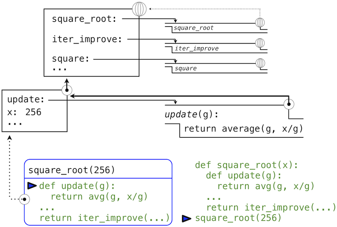
After these nested function definitions, the expression return iter_improve(update, test) in the body of the square_root function needs to be evaluated. The name update, which is passed as an argument to iter_improve , is looked up and resolved to the newly defined function. The same happens for the name test.
With these bindings for update and test , the function call iter_improve(update, test) now gets evaluated. For this evaluation, a new local environment is created where update and test are bound to these functions (again, in the picture below, only update is shown), and where guess is bound to its default value 1. Since iter_improve was defined in the global environment, this local environment points to the global environment, so that it can lookup unresolved names in the environment where the function iter_improve that is being called was originally defined.
Within the body of iter_improve, in the while condition, we must apply the update function to the initial guess of 1. This final application again creates a new local environment for update that contains only a binding of its formal parameter g bound to the value 1.
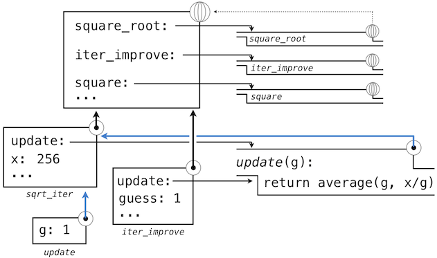
The most crucial part of this evaluation procedure is to find out to what other environment this new local environment should point. This is highlighted by the blue arrows in the diagram. The environment created for the update call, will be scoped within the environment in which update was defined, which can be found by following the blue link back from the update function to its environment of definition (which was the environment created when evaluating square_root(256) and that still contains a binding for x).
In this way, the body of update can resolve a value for x. Hence, we realize two key advantages of lexical scoping in Python.
- The names of a local function do not interfere with names external to the function in which it is defined, because the local function name will be bound in the current local environment in which it is defined, rather than the global environment.
- A local function can access the environment of the enclosing function. This is because the body of the local function is evaluated in an environment that extends the evaluation environment in which it is defined.
The update function thus implicitly carries with it some data: the values referenced in the environment in which it was defined. Because they enclose information in this way, locally defined functions are often called closures.
Functions as Returned Values
We can achieve even more expressive power in our programs by creating functions whose returned values are themselves functions. An important feature of lexically scoped programming languages is that locally defined functions keep their associated environment when they are returned. The following example illustrates the utility of this feature.
With many simple functions defined, function composition is a natural method of combination to include in our programming language. That is, given two functions f(x) and g(x), we might want to define h(x) = f(g(x)). We can define function composition using our existing tools:
def compose1(f, g):
    def h(x):
        return f(g(x))
    return h
>>> add_one_and_square = compose1(square, successor)
>>> add_one_and_square(12)
169
The 1 in compose1 indicates that the composed functions and returned result all take 1 argument. This naming convention isn't enforced by the interpreter; the 1 is just part of the function name.
Lambda Expressions
So far, every time we want to define a new function, we need to give it a name. But for other types of expressions, we don’t need to associate intermediate products with a name. That is, we can compute a*b + c*d without having to name the subexpressions a*b or c*d, or the full expression a*b + c*d. In Python, we can create function values on the fly using lambda expressions, which evaluate to unnamed functions. A lambda expression evaluates to a function that has a single return expression as its body. Assignment and control statements are not allowed.
As opposed to functional programming languages, lambda expressions in Python are quite limited: they are only useful for simple, one-line functions that evaluate and return a single expression. In those special cases where they apply, lambda expressions can be quite expressive, however.
def compose1(f,g):
    return lambda x: f(g(x))
We can understand the structure of a lambda expression by constructing a corresponding English sentence:
lambda              x              :           f(g(x))
"A function that    takes x    and returns     f(g(x))"
Some programmers find that using unnamed functions from lambda expressions is shorter and more direct. However, compound lambda expressions are notoriously illegible, despite their brevity. The following definition is correct, but some programmers have trouble understanding it quickly.
compose1 = lambda f,g: lambda x: f(g(x))
In general, Python style prefers explicit def statements to lambda expressions, but allows them in cases where a simple function is needed as an argument or return value.
Such stylistic rules are merely guidelines; you can program any way you wish. However, as you write programs, think about the audience of people who might read your program one day. If you can make your program easier to interpret, you will do those people a favor.
The term lambda is a historical accident resulting from the incompatibility of written mathematical notation and the constraints of early type-setting systems.
It may seem perverse to use lambda to introduce a procedure/function. The notation goes back to Alonzo Church, who in the 1930's started with a "hat" symbol; he wrote the square function as "ŷ . y × y". But frustrated typographers moved the hat to the left of the parameter and changed it to a capital lambda: "Λy . y × y"; from there the capital lambda was changed to lowercase, and now we see "λy . y × y" in math books and (lambda (y) ( y y)) in Lisp.* ---Peter Norvig (norvig.com/lispy2.html)
Despite their unusual etymology, lambda expressions and the corresponding formal language for function application, the lambda calculus, are fundamental computer science concepts shared far beyond the Python programming community. You will very likely encounter it in other programming languages or other computer science courses.
Example: Newton's Method
This final extended example shows how function values, local definitions, and lambda expressions can work together to express general ideas concisely.
Newton's method is a classic iterative approach to finding the arguments x for which a single-argument mathematical function f(x) yields a return value of 0. In other words, the values of x for which that function f cuts the x-axis (f(x) = 0). These values are called the roots of that function. Finding a root of a single-argument mathematical function is often equivalent to solving a related math problem. For example:
The square root of 16 is the value x such that: square(x) - 16 = 0 .
The logarithm with base 2 of 32 is the value x such that: pow(2, x) - 32 = 0 (i.e., the exponent x to which we would raise 2 to get 32).
Thus, a general method for finding the roots of a function would also provide us an algorithm to compute square roots and logarithms. Moreover, the functions for which we want to compute roots contain simpler operations (multiplication and exponentiation) than the original function we want to compute (square root and logarithm).
A comment before we proceed: it is easy to take for granted the fact that we know how to compute square roots and logarithms. Not just Python, but your phone, your pocket calculator, and perhaps even your watch can do so for you. However, part of learning computer science is understanding how quantities like these can be computed, and the general approach presented here is applicable to solving a large class of equations beyond those built into Python.
Before even beginning to understand Newton's method, we can start programming; this is the power of functional abstractions. We simply translate our previous statements into code.
def square_root(a):
    return find_root(lambda x: square(x) - a)

def logarithm(a, base=2):
    return find_root(lambda x: pow(base, x) - a)
Of course, we cannot apply any of these functions yet until we define find_root, and so we need to understand how Newton's method works.
Like the algorithm we saw before, Newton's method is also an iterative improvement algorithm. It improves a guess of the root for any function that is differentiable (in the mathematical sense). Notice that both of our functions of interest change smoothly; graphing x versus f(x) for
f(x) = square(x) - 16 (light curve)
f(x) = pow(2, x) - 32 (dark curve)
on a 2-dimensional plane shows that both functions produce a smooth curve without kinks that crosses the x-axis (f(x)=0) at the appropriate point.
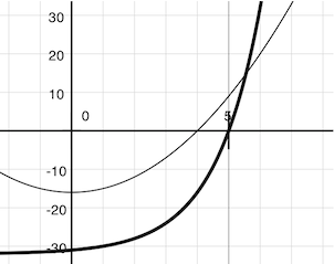
Because they are smooth (differentiable), these curves can be approximated by a line at any point. Newton's method follows these linear approximations to find function roots.
Imagine a line through the point (x, f(x)) that has the same slope as the curve for function f(x) at that point. Such a line is called the tangent, and its slope is called the derivative of f at x.
This line's slope is the ratio of the change in function value to the change in function argument. Hence, translating x by f(x) divided by the slope will give the argument value at which this tangent line touches 0.
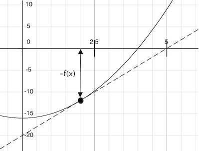
Our newton_update function expresses the computational process of following this tangent line to 0. We approximate the derivative of the function by computing its slope over a very small interval.
def approx_derivative(f, x, delta=1e-5):
    df = f(x + delta) - f(x)
    return df/delta

def newton_update(f):
    def update(x):
        return x - f(x) / approx_derivative(f, x)
    return update
Finally, we can define the find_root function in terms of newton_update, our iterative improvement algorithm, and a test to see if f(x) is near 0. We supply a larger initial guess to improve the performance for logarithm.
def find_root(f, initial_guess=10):
    def test(x):
        return approx_eq(f(x), 0)
    return iter_improve(newton_update(f), test, initial_guess)
>>> square_root(16)
4.000000000026422

>>> logarithm(32, 2)
5.000000094858201
And to verify that these values are correct, you can test:
>>> square(square_root(16))
16.00000000021138
>>> pow(2,logarithm(32, 2))
32.0000021040223
As you experiment with Newton's method, be aware that it will not always converge. The initial guess of iter_improve must be sufficiently close to the root, and various conditions about the function must be met. Despite this shortcoming, Newton's method is a powerful general computational method for solving differentiable equations. In fact, very fast algorithms for logarithms and large integer division employ variants of the technique.
Abstractions and First-Class Functions
We began this section with the observation that user-defined functions are a crucial abstraction mechanism, because they permit us to express general methods of computing as explicit elements in our programming language. Now we've seen how higher-order functions permit us to manipulate these general methods to create further abstractions.
As programmers, we should be alert to opportunities to identify the underlying abstractions in our programs, to build upon them, and generalize them to create more powerful abstractions. This is not to say that one should always write programs in the most abstract way possible; expert programmers know how to choose the level of abstraction appropriate to their task. But it is important to be able to think in terms of these abstractions, so that we can be ready to apply them in new contexts. The significance of higher-order functions is that they enable us to represent these abstractions explicitly as elements in our programming language, so that they can be handled just like other computational elements.
In general, programming languages impose restrictions on the ways in which computational elements can be manipulated. Elements with the fewest restrictions are said to have first-class status. Some of the "rights and privileges" of first-class language elements are:
- They may be bound to names.
- They may be passed as arguments to functions.
- They may be returned as the results of functions.
- They may be included in data structures.
Python awards functions full first-class status, and the resulting gain in expressive power is enormous. Control structures, on the other hand, do not: you cannot pass if to a function the way you can sum.
Function Decorators
Python provides special syntax to apply higher-order functions as part of executing a def statement, called a decorator. Perhaps the most common example is a trace.
def trace1(f):
    def wrapped(x):
        print('-> ', f, '(', x, ')')
        return f(x)
    return wrapped

@trace1
def triple(x):
    return 3 * x
>>> triple(12)
-> <function triple at 0x102a39848> ( 12 )
36
In this example, a higher-order function trace1 is defined, which returns a function that precedes a call to its argument with a print statement that outputs the argument. The def statement for triple has an annototation, @trace1, which affects the execution rule for def. As usual, the function triple is created. However, the name triple is not bound to this function. Instead, the name triple is bound to the returned function value of calling trace1 on the newly defined triple function. In fact, in code this decorator is equivalent to:
def triple(x):
    return 3 * x

triple = trace1(triple)
If you want, try and apply the @trace1 annotation to the Fibonacci function fib(n) before calling it with some value of n, to observe to how many recursive calls it leads.
@trace1
def fib(n):
    if n <= 1:
        return n
    return fib(n-1) + fib(n-2)

fib(10)
>>> fib(5)
-> <function fib at 0x104147d90> ( 5 )
-> <function fib at 0x104147d90> ( 4 )
-> <function fib at 0x104147d90> ( 3 )
-> <function fib at 0x104147d90> ( 2 )
-> <function fib at 0x104147d90> ( 1 )
-> <function fib at 0x104147d90> ( 0 )
-> <function fib at 0x104147d90> ( 1 )
-> <function fib at 0x104147d90> ( 2 )
-> <function fib at 0x104147d90> ( 1 )
-> <function fib at 0x104147d90> ( 0 )
-> <function fib at 0x104147d90> ( 3 )
-> <function fib at 0x104147d90> ( 2 )
-> <function fib at 0x104147d90> ( 1 )
-> <function fib at 0x104147d90> ( 0 )
-> <function fib at 0x104147d90> ( 1 )
5
Decorators can be used for tracing, for selecting which functions to call when a program is run from the command line, and many other things.
Extra for experts. The actual rule is that the decorator symbol @ may be followed by an expression (@trace1 is just a simple expression consisting of a single name). Any expression producing a suitable value is allowed. For example, with a suitable definition, you could define a decorator check_range so that decorating a function definition with @check_range(1, 10) would cause the function's results to be checked to make sure they are integers between 1 and 10. The call check_range(1,10) would return a function that would then be applied to the newly defined function before it is bound to the name in the def statement.
Glossary
- higher-order functions
- Higher-order functions are functions that can accept other functions as arguments or that return functions as values.
- general methods of computation
- Higher-order functions can serve as powerful abstraction mechanisms to express general methods of computation, independent of the particular functions they call. These higher-order functions can then be supplied with particular functions to produce more specific computations. For example, a higher-order function that expresses the high-level computational process of iterative improvement, could be customized, by providing the right functions as arguments, into a method for computing an approximation of the golden ratio.
- nested functions
- Nested function definitions are functions that are defined locally in the body of another function definition. Nested function definitions have two main advantages. Firstly, because the functions are defined locally, they don't clutter the global namespace with the names of many small auxiliary functions. Secondly, since the functions are scoped within the body of another function, they have access to all parameters and variables declared locally inside that other function. Because of that, those nested functions often require less parameters than if they would have been defined globally.
- lexical scope
- The discipline of sharing names among nested definitions is called lexical scoping: all nested function definitions have access to the names visible in their environment of definition (as opposed to the environment where they were called).
- nested scope
- Since function definitions can be nested inside other function definitions, which can again be nested inside other function definitions, we can have multiple layers of nested lexical scopes. In such cases, name resolution (i.e., the process of looking up names for variables or functions) will proceed layer by layer from the inner-most scope where a function was defined until it eventually reaches the outermost global namespace.
- shadowing
- Related to nested scopes, shadowing refers to a situation where two (variable or function) names exist within scopes that overlap. Whenever that happens, the name with the outermost scope is hidden because the variable with the more nested scope overrides it. The outermost variable is said to be shadowed by the innermost one.
- function as returned value
- In Python, just like it is possible to create functions that take other functions are arguments, it is possible to write functions whose returned values are themselves functions.
- lambda expression
- Lambda expressions are a way to define new functions, without needing to give them a name. A lambda expression evaluates to a function that has a single return expression as its body. Lambda expressions in Python are quite limited: they are only useful for simple, one-line functions that evaluate and return a single expression. Assignment and control statements are not allowed.
- first-class functions
- In general, programming languages impose restrictions on how certain language elements can be manipulated. Elements with the fewest restrictions are said to have first-class status. Some of the "rights and privileges" of first-class language element are that they can be bound to names, be passed as arguments to functions, be returned as the results of functions and that they may be included in data structures. Since all this is the case for functions in Python, functions are first-class elements in Python.
- function decorators
- By definition, a function decorator is a function that takes another function and extends the behavior of the latter function without explicitly modifying it. Function decorators provide a simple syntax for calling higher-order functions, by simply annotating the definition of a function with the higher-order function that needs to be applied to it upon calling that function.
References
| [SICP] | SICP in Python. This book is derived from the classic textbook "Structure and Interpretation of Computer Programs" by Abelson, Sussman, and Sussman. John Denero originally modified it for Python in 2011. It is licensed under the Creative Commons Attribution-ShareAlike 3.0 license. |
| [ThinkCS] | How To Think Like a Computer Scientist --- Learning with Python 3 |
| [GoldenRatio] | (1, 2, 3) https://en.wikipedia.org/wiki/Golden_ratio |