Recursion
Source: this section is heavily based on Chapter 18 of [ThinkCS].
Recursion means "defining something in terms of itself" usually at some smaller scale, perhaps multiple times, to achieve some objective. For example, we might say "A human being is someone whose parents are human beings", or "a directory is a structure that holds files and (smaller) directories", or "a family tree starts with a couple who have children, each with their own family sub-trees".
Programming languages generally support recursion, which means that, in order to solve a problem, functions can call themselves to solve smaller subproblems.
Drawing Fractals
A fractal is a drawing that has self-similar structure, which can be defined in terms of itself. [Fractal]
Let us start by looking at the famous Koch fractal. An order 0 Koch fractal is simply a straight line of a given size.
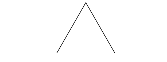
An order 1 Koch fractal is obtained like this: instead of drawing just one line, draw instead four smaller segments, as in the pattern shown below.
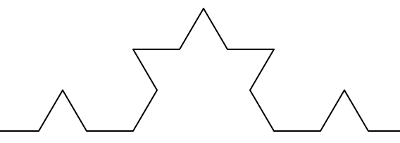
Now what would happen if we repeated this Koch pattern again on each of the order 1 segments? We'd get an order 2 Koch fractal.
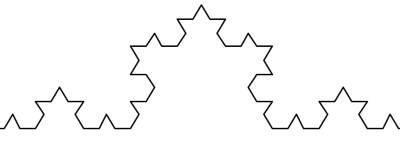
Repeating our pattern again gets us an order 3 Koch fractal.
And so on, and so forth. For example this is an order 5 Koch fractal.
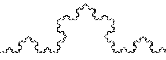
Now let us think about it the other way around. To draw a Koch fractal of order 3, we can simply draw four order 2 Koch fractals. But each of these in turn needs four order 1 Koch fractals, and each of those in turn needs four order 0 fractals. Ultimately, the only drawing that will take place is at order 0. This is very simple to code up in Python:
def koch(t, order, size):
    """
       Makes turtle 't' draw a Koch fractal of 'order' and 'size'.
       pre:  't' is a Turtle object, ready to draw on some Screen
       post: A Koch fractal of given 'order' and 'size' has been
             drawn by turtle 't' on the screen, and the turtle 't'
             is left facing the same direction.
    """

    if order == 0:          # The base case is just a straight line
        t.forward(size)
    else:
        koch(t, order-1, size/3)   # Go 1/3 of the way
        t.left(60)
        koch(t, order-1, size/3)
        t.right(120)
        koch(t, order-1, size/3)
        t.left(60)
        koch(t, order-1, size/3)

"Of course, to actually run the code above we still need to"
"add the necessary instructions to set up the turtle graphics:"

import turtle
window = turtle.Screen()
t = turtle.Turtle()
t.speed(0)
t.penup()
t.forward(-150)
t.pendown()
koch(t,5,300)     # <- Here is the actual call to the koch function !
window.mainloop()
The key thing that is new here is that as long as order is not zero, koch calls itself recursively to get its job done.
Rereading the above code of the koch function, we observe that it contains a quite repetitive pattern. (Do you see it?) Not quite fond of duplicated code, we will try to tighten up the code a bit to get rid of this repetition. First of all, remember that turning right by 120 degrees is the same as turning left by -120 degrees. So with a bit of clever rearrangement, we can use a single loop to make the four recursive calls to the koch function in the else-branch.
def koch(t, order, size):
    if order == 0:
        t.forward(size)
    else:
        for angle in [60, -120, 60, 0]:
           koch(t, order-1, size/3)
           t.left(angle)
The final turn is 0 degrees, so it has no effect. But it has allowed us to find a pattern and reduce seven lines of code to three, which will make things easier for our next observations.
Recursion, the high-level view
One way to think about this is to convince yourself that the function works correctly when you call it for an order 0 fractal. Then do a mental leap of faith, saying "I will assume that Python will handle correctly the four recursive level 0 calls for me in the else-branch, so I don't need to think about that detail. So all I need to focus on now is how to draw an order 1 fractal assuming that the order 0 one is already working."
You're practicing mental abstraction --- ignoring the subproblem while you solve the big problem.
If this mode of thinking works (and you should practice it!), then take it to the next level. Aha! now can I see that it will work when called for order 2 under the assumption that it is already working for level 1.
And, in general, if I can assume the order n-1 case works, can I just solve the level n problem?
Students of mathematics who have played with proofs of induction should see some very strong similarities here.
Recursion, the low-level operational view
Another way of trying to understand recursion is to get rid of it! If we had separate functions to draw a level 3 fractal, a level 2 fractal, a level 1 fractal and a level 0 fractal, we could simplify the above code, quite mechanically, to a situation where there was no longer any recursion, like this:
def koch_0(t, size):
    t.forward(size)

def koch_1(t, size):
    for angle in [60, -120, 60, 0]:
       koch_0(t, size/3)
       t.left(angle)

def koch_2(t, size):
    for angle in [60, -120, 60, 0]:
       koch_1(t, size/3)
       t.left(angle)

def koch_3(t, size):
    for angle in [60, -120, 60, 0]:
       koch_2(t, size/3)
       t.left(angle)
This trick of "unfolding" the recursion gives us an operational view of what happens. You can trace the program into koch_3, and from there, into koch_2, and then into koch_1, etc., all the way down the different layers of the recursion.
This might be a useful hint to build your understanding. The mental goal is, however, to be able to do the abstraction!
Recursive data structures
All of the Python data types we have seen can be grouped inside lists and tuples in a variety of ways. Lists and tuples can also be nested, providing many possibilities for organizing data. The organization of data for the purpose of making it easier to use is called a data structure.
Suppose it is election time and that we are helping to count votes as they come in. Votes arriving from individual districts, cities, agglomerations and provinces are sometimes reported as a sum total of votes and sometimes as a list of subtotals of votes. After considering how best to store this incoming data, we decide to use a nested number list, which we define as follows:
A nested number list is a list whose elements are either:
- numbers
- nested number lists
Notice how in the above definition, the term nested number list is used to define itself. Recursive definitions like this are quite common in mathematics and computer science. They provide a concise and powerful way to describe recursive data structures that are partially composed of smaller and simpler instances of themselves. The definition is not circular, nor infinite, since at some point we will reach a list that does not have any lists as elements.
Now suppose our job is to write a function that will sum all of the values in a nested number list. Python has a built-in function which finds the sum of a sequence of numbers:
>>> sum([1, 2, 8])
11
For our nested number list, however, sum will not work:
>>> sum([1, 2, [11, 13], 8])
Traceback (most recent call last):
  File "<pyshell>", line 1, in <module>
TypeError: unsupported operand type(s) for +: 'int' and 'list'
The problem is that the third element of this list, [11, 13], is itself a list, so it cannot just be added to 1, 2, and 8.
Processing recursive number lists
To sum all the numbers in our recursive nested number list we need to traverse the list, visiting each of the elements within its nested structure, adding any numeric elements to our sum, and recursively repeating the summing process with any elements which are themselves sub-lists.
Thanks to recursion, the Python code needed to sum the values of a nested number list is surprisingly short:
def r_sum(nested_num_list):
    """
      Computes the sum of all values in a recursively nested structure of lists.
      pre:  'nested_num_list' is a nested number list, i.e., a list whose elements
            are either numbers or again nested number lists.
      post: returns 0 for empty lists or the sum of all encountered values,
            at any level of nesting, for nested number lists.
    """
    tot = 0
    for element in nested_num_list:
        if isinstance(element,list):
            tot += r_sum(element)
        else:
            tot += element
    return tot
>>> r_sum([1, 2, [11, 13], 8])
35
The body of r_sum consists mainly of a for loop that traverses nested_num_list. If element is a numerical value (the else branch), it is simply added to tot. If element is a list (which is checked with the type check isinstance(element,list)), then r_sum is called again, with the element as an argument. The statement inside the function definition in which the function calls itself is known as the recursive call.
The example above has a base case (the else branch) which does not lead to a recursive call: the case where the element is not a (sub-) list. Without a base case, you'll have infinite recursion, and your program will not work.
Recursion is truly one of the most beautiful and elegant tools in computer science.
A slightly more complicated problem is finding the largest value in a nested number list:
def r_max(nxs):
    """
      Finds the maximum value in a recursively nested structure of lists.
      pre:  'nxs' is a nested number list, i.e., a list whose elements
            are either numbers or again nested number lists.
            No lists or sublists are empty.
      post: returns the maximum value of all encountered values
            in this nested structure of lists.
    """
    largest = None
    first_time = True
    for e in nxs:
        if isinstance(e,list):
            val = r_max(e)
        else:
            val = e

        if first_time or val > largest:
            largest = val
            first_time = False

    return largest

test(r_max([2, 9, [1, 13], 8, 6]) == 13)
test(r_max([2, [[100, 7], 90], [1, 13], 8, 6]) == 100)
test(r_max([[[13, 7], 90], 2, [1, 100], 8, 6]) == 100)
test(r_max(["joe", ["sam", "ben"]]) == "sam")
We included some tests to provide examples of r_max at work. (All these assertions should succeed. Figure out for yourself what would happen if the list or one of its nested sublists would be empty.)
The added twist to this problem is finding a value for initializing largest. We can't just use nxs[0], since that could be either an element or a list. To solve this problem (at every recursive call) we set a Boolean flag first_time to True (at line 11). When we've found the value of interest (at line 17), we check to see whether this is the initializing (first) value for largest, or a value that could potentially change largest.
Again here we have a base case at line 15. If we don't supply a base case, Python stops after reaching a maximum recursion depth and returns a runtime error. See how this happens, by running this little script which we will call infinite_recursion.py:
def recursion_depth(number):
    print("{0}, ".format(number), end="")
    recursion_depth(number + 1)

recursion_depth(0)
After watching the messages flash by, you will be presented with the end of a long traceback that ends with a message like the following:
RecursionError: maximum recursion depth exceeded while calling a Python object
We would certainly never want something like this to happen to a user of one of our programs, so it is good programming practice to write error handling code that could handle such errors when they arise.
Fibonacci numbers
The famous Fibonacci sequence 0, 1, 1, 2, 3, 5, 8, 13, 21, 34, 55, 89, 144, ... [FibonacciNumber] was devised by Fibonacci (1170-1250), who used this to model the breeding of (pairs) of rabbits. If, in generation 8 you had 21 pairs in total, of which 13 were adults, then next generation the adults will all have bred new children, and the previous children will have grown up to become adults. So in generation 9 you'll have 13+21=34, of which 21 are adults.
This model to explain rabbit breeding made the simplifying assumption that rabbits never died. Scientists often make (over-)simplifying assumptions and restrictions to make some headway with the problem.
If we number the terms of the sequence from 0, we can describe each term recursively as the sum of the previous two terms:
fib(0) = 0
fib(1) = 1
fib(n) = fib(n-1) + fib(n-2)  for n >= 2
This translates very directly into some Python:
def fib(n):
    """
      Computes numbers in the Fibonacci sequence 0, 1, 1, 2, 3, 5, 8, 13, 21, ...
      pre:  'n' is natural number (an integer >= 0)
      post: returns the n-th Fibonacci number,
            where fib(0) = 0 and fib(1) = 1
            and any other Fibonacci number is defined
            as the sum of the previous 2 Fibonacci numbers,
            for example: fib(2) = fib(0) + fib(1) = 0 + 1 = 1
    """
    if n <= 1:
        return n
    t = fib(n-1) + fib(n-2)
    return t

test(fib(0) == 0)
test(fib(1) == 1)
test(fib(2) == 1)
test(fib(3) == 2)
test(fib(4) == 3)
test(fib(5) == 5)
test(fib(6) == 8)
test(fib(7) == 13)
test(fib(8) == 21)
test(fib(9) == 34)
test(fib(10) == 55)
test(fib(11) == 89)
test(fib(12) == 144)
This is a particularly inefficient algorithm. One particular way of fixing this inefficiency, which we will leave as an exercise for now, is to make use of dictionaries to remember (or memoize) previously calculated values of the function so that they don't need to be recalculated over and over again.
import time
from time import process_time
t0 = process_time()
n = 35
result = fib(n)
t1 = process_time()

print("fib({0}) = {1}, ({2:.2f} secs)".format(n, result, t1-t0))
We get the correct result, but an exploding amount of work!
fib(35) = 9227465, (4.51 secs)
Memoization
If you play around a bit with the fib function from the previous section, you will notice that the bigger the argument you provide, the longer the function takes to run. Furthermore, the run time increases very quickly. On one of our machines, fib(20) finishes instantly, fib(30) takes about a second, and fib(40) takes roughly forever.
To understand why, consider this call graph for fib with n = 4:
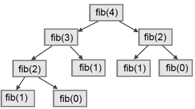
A call graph shows some function frames (instances when the function has been invoked), with lines connecting each frame to the frames of the functions it calls. At the top of the graph, fib with n = 4 calls fib with n = 3 and n = 2. In turn, fib with n = 3 calls fib with n = 2 and n = 1. And so on.
Count how many times fib(0) and fib(1) are called. This is an inefficient solution to the problem, and it gets far worse as the argument gets bigger.
A good solution is to keep track of values that have already been computed by storing them in a dictionary. A previously computed value that is stored for later use is called a memo. Here is an implementation of fib using memos:
alreadyknown = {0: 0, 1: 1}

def fib(n):
    if n not in alreadyknown:
        new_value = fib(n-1) + fib(n-2)
        alreadyknown[n] = new_value
    return alreadyknown[n]
The dictionary named alreadyknown keeps track of the Fibonacci numbers we already know. We start with only two pairs: 0 maps to 1; and 1 maps to 1.
Whenever fib is called, it checks the dictionary to determine if it contains the result. If it's there, the function can return immediately without making any more recursive calls. If not, it has to compute the new value. The new value is added to the dictionary before the function returns.
Using this version of fib, our machines can compute fib(100) in an eyeblink.
>>> fib(100)
354224848179261915075
Example with recursive directories and files
The following program lists the contents of a directory and all its subdirectories. Notice how a recursive function print_files is used to recursively walk through the recursively nested directory structure.
import os

def get_dirlist(path):
    """
      Produces the list of all files in a given directory.
      pre:  'path' is a string describing a valid path to a directory
            in the operating system.
      post: Returns a sorted list of the names of all entries (files
            or directories) encountered in the directory with that path.
            This returns just the names, not the full path to the names.
            Directories nested in this directory are not recursively explored.
    """
    dirlist = os.listdir(path)
    dirlist.sort()
    return dirlist

def print_files(path, prefix = ""):
    """
      Prints the recursive listing of all contents in a given directory.
      pre:  'path' is a string describing a valid path to a directory
            in the operating system.
      post: Prints the path and the names of all entries (files or directories
            contained in it). Nested directories are visited recursively.
            For every entry, the nesting level is indicated by vertical bars.
            Entries directly contained in the path are preceded by one bar,
            entries at nesting level 2 by two bars, and so on.
    """
    if prefix == "":  # Detect outermost call, print a heading
        print("Folder listing for", path)
        prefix = "| "

    dirlist = get_dirlist(path)
    for f in dirlist:
        print(prefix+f)                    # Print the line
        fullname = os.path.join(path, f)   # Turn name into full pathname
        if os.path.isdir(fullname):        # If a directory, recurse.
            print_files(fullname, prefix + "| ")
Calling the function print_files with some initial path or folder name will produce an output similar to this:
print_files("c:\python31\Lib\site-packages\pygame\examples")

Folder listing for c:\python31\Lib\site-packages\pygame\examples
| __init__.py
| aacircle.py
| aliens.py
| arraydemo.py
| blend_fill.py
| blit_blends.py
| camera.py
| chimp.py
| cursors.py
| data
| | alien1.png
| | alien2.png
| | alien3.png
...
Glossary
- base case
- A branch of the conditional statement in a recursive function that does not give rise to further recursive calls.
- infinite recursion
- A function that calls itself recursively without ever reaching any base case. Eventually, infinite recursion causes a runtime error.
- recursion
- The process of calling a function that is already executing.
- recursive call
- The statement that calls an already executing function. Recursion can also be indirect --- function f can call g which calls h, and h could make a call back to f --- or mutual --- function f calls g and g makes a call back to f.
- recursive definition
- A definition which defines something in terms of itself. To be useful it must include base cases which are not recursive. In this way it differs from a circular definition. Recursive definitions often provide an elegant way to express complex data structures, like a directory that can contain other directories, or a menu that can contain other menus.
References
| [ThinkCS] | How To Think Like a Computer Scientist --- Learning with Python 3 |
| [Fractal] | https://en.wikipedia.org/wiki/Fractal |
| [FibonacciNumber] | https://en.wikipedia.org/wiki/Fibonacci_number |