Table des matières
Introduction
The way of the program
Source: this section is heavily based on Chapter 1 of [ThinkCS].
The goal of this book is to teach you to think like a computer scientist. This way of thinking combines some of the best features of mathematics, engineering, and natural science. Like mathematicians, computer scientists use formal languages to denote ideas (specifically computations). Like engineers, they design things, assembling components into systems and evaluating tradeoffs among alternatives. Like scientists, they observe the behavior of complex systems, form hypotheses, and test predictions.
The single most important skill for a computer scientist is problem solving. Problem solving means the ability to formulate problems, think creatively about solutions, and express a solution clearly and accurately. As it turns out, the process of learning to program is an excellent opportunity to practice problem-solving skills. That's why this chapter is called, The way of the program.
On one level, you will be learning to program, a useful skill by itself. On another level, you will use programming as a means to an end. As we go along, that end will become clearer.
The Python programming language
The programming language you will be learning is Python. Python is an example of a high-level language; other high-level languages you might have heard of are C++, PHP, Pascal, C#, and Java.
As you might infer from the name high-level language, there are also low-level languages, sometimes referred to as machine languages or assembly languages. Loosely speaking, computers can only execute programs written in low-level languages. Thus, programs written in a high-level language have to be translated into something more suitable before they can run.
Almost all programs are written in high-level languages because of their advantages. It is much easier to program in a high-level language so programs take less time to write, they are shorter and easier to read, and they are more likely to be correct. Second, high-level languages are portable, meaning that they can run on different kinds of computers with few or no modifications.
The engine that translates and runs Python is called the Python Interpreter: There are two ways to use it: immediate mode and script mode. In immediate mode, you type Python expressions into the Python Interpreter window, and the interpreter immediately shows the result:
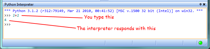
The >>> is called the Python prompt. The interpreter uses the prompt to indicate that it is ready for instructions. We typed 2 + 2, and the interpreter evaluated our expression, and replied 4, and on the next line it gave a new prompt, indicating that it is ready for more input.
Alternatively, you can write a program in a file and use the interpreter to execute the contents of the file. Such a file is called a script. Scripts have the advantage that they can be saved to disk, printed, and so on.
In this Rhodes Local Edition of the textbook, we use a program development environment called PyScripter. (It is available at http://code.google.com/p/pyscripter.) There are various other development environments. If you're using one of the others, you might be better off working with the authors' original book rather than this edition.
For example, we created a file named firstprogram.py using PyScripter. By convention, files that contain Python programs have names that end with .py
To execute the program, we can click the Run button in PyScripter:
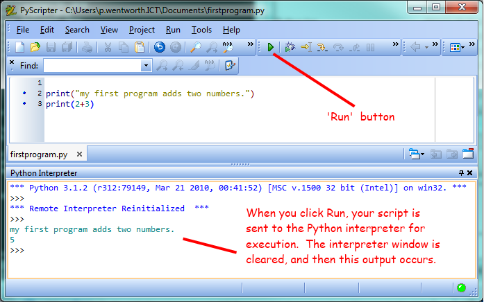
Most programs are more interesting than this one.
Working directly in the interpreter is convenient for testing short bits of code because you get immediate feedback. Think of it as scratch paper used to help you work out problems. Anything longer than a few lines should be put into a script.
What is a program?
A program is a sequence of instructions that specifies how to perform a computation. The computation might be something mathematical, such as solving a system of equations or finding the roots of a polynomial, but it can also be a symbolic computation, such as searching and replacing text in a document or (strangely enough) compiling a program.
The details look different in different languages, but a few basic instructions appear in just about every language:
- input
- Get data from the keyboard, a file, or some other device.
- output
- Display data on the screen or send data to a file or other device.
- math
- Perform basic mathematical operations like addition and multiplication.
- conditional execution
- Check for certain conditions and execute the appropriate sequence of statements.
- repetition
- Perform some action repeatedly, usually with some variation.
Believe it or not, that's pretty much all there is to it. Every program you've ever used, no matter how complicated, is made up of instructions that look more or less like these. Thus, we can describe programming as the process of breaking a large, complex task into smaller and smaller subtasks until the subtasks are simple enough to be performed with sequences of these basic instructions.
That may be a little vague, but we will come back to this topic later when we talk about algorithms.
What is debugging?
Programming is a complex process, and because it is done by human beings, it often leads to errors. Programming errors are called bugs and the process of tracking them down and correcting them is called debugging. Use of the term bug to describe small engineering difficulties dates back to at least 1889, when Thomas Edison had a bug with his phonograph.
Three kinds of errors can occur in a program: syntax errors, runtime errors, and semantic errors. It is useful to distinguish between them in order to track them down more quickly.
Syntax errors
Python can only execute a program if the program is syntactically correct; otherwise, the process fails and returns an error message. Syntax refers to the structure of a program and the rules about that structure. For example, in English, a sentence must begin with a capital letter and end with a period. this sentence contains a syntax error. So does this one
For most readers, a few syntax errors are not a significant problem, which is why we can read the poetry of E. E. Cummings without problems. Python is not so forgiving. If there is a single syntax error anywhere in your program, Python will display an error message and quit, and you will not be able to run your program. During the first few weeks of your programming career, you will probably spend a lot of time tracking down syntax errors. As you gain experience, though, you will make fewer errors and find them faster.
Runtime errors
The second type of error is a runtime error, so called because the error does not appear until you run the program. These errors are also called exceptions because they usually indicate that something exceptional (and bad) has happened.
Runtime errors are rare in the simple programs you will see in the first few chapters, so it might be a while before you encounter one.
Semantic errors
The third type of error is the semantic error. If there is a semantic error in your program, it will run successfully, in the sense that the computer will not generate any error messages, but it will not do the right thing. It will do something else. Specifically, it will do what you told it to do.
The problem is that the program you wrote is not the program you wanted to write. The meaning of the program (its semantics) is wrong. Identifying semantic errors can be tricky because it requires you to work backward by looking at the output of the program and trying to figure out what it is doing.
Experimental debugging
One of the most important skills you will acquire is debugging. Although it can be frustrating, debugging is one of the most intellectually rich, challenging, and interesting parts of programming.
In some ways, debugging is like detective work. You are confronted with clues, and you have to infer the processes and events that led to the results you see.
Debugging is also like an experimental science. Once you have an idea what is going wrong, you modify your program and try again. If your hypothesis was correct, then you can predict the result of the modification, and you take a step closer to a working program. If your hypothesis was wrong, you have to come up with a new one. As Sherlock Holmes pointed out, When you have eliminated the impossible, whatever remains, however improbable, must be the truth. (A. Conan Doyle, The Sign of Four)
For some people, programming and debugging are the same thing. That is, programming is the process of gradually debugging a program until it does what you want. The idea is that you should start with a program that does something and make small modifications, debugging them as you go, so that you always have a working program.
For example, Linux is an operating system kernel that contains millions of lines of code, but it started out as a simple program Linus Torvalds used to explore the Intel 80386 chip. According to Larry Greenfield, one of Linus's earlier projects was a program that would switch between displaying AAAA and BBBB. This later evolved to Linux (The Linux Users' Guide Beta Version 1).
Later chapters will make more suggestions about debugging and other programming practices.
Formal and natural languages
Natural languages are the languages that people speak, such as English, Spanish, and French. They were not designed by people (although people try to impose some order on them); they evolved naturally.
Formal languages are languages that are designed by people for specific applications. For example, the notation that mathematicians use is a formal language that is particularly good at denoting relationships among numbers and symbols. Chemists use a formal language to represent the chemical structure of molecules. And most importantly:
Programming languages are formal languages that have been designed to express computations.
Formal languages tend to have strict rules about syntax. For example, 3+3=6 is a syntactically correct mathematical statement, but 3=+6$ is not. H2O is a syntactically correct chemical name, but 2Zz is not.
Syntax rules come in two flavors, pertaining to tokens and structure. Tokens are the basic elements of the language, such as words, numbers, parentheses, commas, and so on. In Python, a statement like print("Happy New Year for ",2013) has 6 tokens: a function name, an open parenthesis (round bracket), a string, a comma, a number, and a close parenthesis.
It is possible to make errors in the way one constructs tokens. One of the problems with 3=+6$ is that $ is not a legal token in mathematics (at least as far as we know). Similarly, 2Zz is not a legal token in chemistry notation because there is no element with the abbreviation Zz.
The second type of syntax rule pertains to the structure of a statement--- that is, the way the tokens are arranged. The statement 3=+6$ is structurally illegal because you can't place a plus sign immediately after an equal sign. Similarly, molecular formulas have to have subscripts after the element name, not before. And in our Python example, if we omitted the comma, or if we changed the two parentheses around to say print)"Happy New Year for ",2013( our statement would still have six legal and valid tokens, but the structure is illegal.
When you read a sentence in English or a statement in a formal language, you have to figure out what the structure of the sentence is (although in a natural language you do this subconsciously). This process is called parsing.
For example, when you hear the sentence, "The other shoe fell", you understand that the other shoe is the subject and fell is the verb. Once you have parsed a sentence, you can figure out what it means, or the semantics of the sentence. Assuming that you know what a shoe is and what it means to fall, you will understand the general implication of this sentence.
Although formal and natural languages have many features in common --- tokens, structure, syntax, and semantics --- there are many differences:
- ambiguity
- Natural languages are full of ambiguity, which people deal with by using contextual clues and other information. Formal languages are designed to be nearly or completely unambiguous, which means that any statement has exactly one meaning, regardless of context.
- redundancy
- In order to make up for ambiguity and reduce misunderstandings, natural languages employ lots of redundancy. As a result, they are often verbose. Formal languages are less redundant and more concise.
- literalness
- Formal languages mean exactly what they say. On the other hand, natural languages are full of idiom and metaphor. If someone says, "The other shoe fell", there is probably no shoe and nothing falling. You'll need to find the original joke to understand the idiomatic meaning of the other shoe falling. Yahoo! Answers thinks it knows!
People who grow up speaking a natural language---everyone---often have a hard time adjusting to formal languages. In some ways, the difference between formal and natural language is like the difference between poetry and prose, but more so:
- poetry
- Words are used for their sounds as well as for their meaning, and the whole poem together creates an effect or emotional response. Ambiguity is not only common but often deliberate.
- prose
- The literal meaning of words is more important, and the structure contributes more meaning. Prose is more amenable to analysis than poetry but still often ambiguous.
- program
- The meaning of a computer program is unambiguous and literal, and can be understood entirely by analysis of the tokens and structure.
Here are some suggestions for reading programs (and other formal languages). First, remember that formal languages are much more dense than natural languages, so it takes longer to read them. Also, the structure is very important, so it is usually not a good idea to read from top to bottom, left to right. Instead, learn to parse the program in your head, identifying the tokens and interpreting the structure. Finally, the details matter. Little things like spelling errors and bad punctuation, which you can get away with in natural languages, can make a big difference in a formal language.
The first program
Traditionally, the first program written in a new language is called Hello, World! because all it does is display the words, Hello, World! In Python, the script looks like this: (For scripts, we'll show line numbers to the left of the Python statements.)
print("Hello, World!")
This is an example of using the print function, which doesn't actually print anything on paper. It displays a value on the screen. In this case, the result shown is
Hello, World!
The quotation marks in the program mark the beginning and end of the value; they don't appear in the result.
Some people judge the quality of a programming language by the simplicity of the Hello, World! program. By this standard, Python does about as well as possible.
Comments
As programs get bigger and more complicated, they get more difficult to read. Formal languages are dense, and it is often difficult to look at a piece of code and figure out what it is doing, or why.
For this reason, it is a good idea to add notes to your programs to explain in natural language what the program is doing.
A comment in a computer program is text that is intended only for the human reader --- it is completely ignored by the interpreter.
In Python, the # token starts a comment. The rest of the line is ignored. Here is a new version of Hello, World!.
#---------------------------------------------------
# This demo program shows off how elegant Python is!
# Written by Joe Soap, December 2010.
# Anyone may freely copy or modify this program.
#---------------------------------------------------

print("Hello, World!")     # Isn't this easy!
You'll also notice that we've left a blank line in the program. Blank lines are also ignored by the interpreter, but comments and blank lines can make your programs much easier for humans to parse. Use them liberally!
Glossary
- algorithm
- A set of specific steps for solving a category of problems.
- bug
- An error in a program.
- comment
- Information in a program that is meant for other programmers (or anyone reading the source code) and has no effect on the execution of the program.
- debugging
- The process of finding and removing any of the three kinds of programming errors.
- exception
- Another name for a runtime error.
- formal language
- Any one of the languages that people have designed for specific purposes, such as representing mathematical ideas or computer programs; all programming languages are formal languages.
- high-level language
- A programming language like Python that is designed to be easy for humans to read and write.
- immediate mode
- A style of using Python where we type expressions at the command prompt, and the results are shown immediately. Contrast with script, and see the entry under Python shell.
- interpreter
- The engine that executes your Python scripts or expressions.
- low-level language
- A programming language that is designed to be easy for a computer to execute; also called machine language or assembly language.
- natural language
- Any one of the languages that people speak that evolved naturally.
- object code
- The output of the compiler after it translates the program.
- parse
- To examine a program and analyze the syntactic structure.
- portability
- A property of a program that can run on more than one kind of computer.
- print function
- A function used in a program or script that causes the Python interpreter to display a value on its output device.
- problem solving
- The process of formulating a problem, finding a solution, and expressing the solution.
- program
- a sequence of instructions that specifies to a computer actions and computations to be performed.
- Python shell
- An interactive user interface to the Python interpreter. The user of a Python shell types commands at the prompt (>>>), and presses the return key to send these commands immediately to the interpreter for processing. The word shell comes from Unix. In the PyScripter used in this RLE version of the book, the Interpreter Window is where we'd do the immediate mode interaction.
- runtime error
- An error that does not occur until the program has started to execute but that prevents the program from continuing.
- script
- A program stored in a file (usually one that will be interpreted).
- semantic error
- An error in a program that makes it do something other than what the programmer intended.
- semantics
- The meaning of a program.
- source code
- A program in a high-level language before being compiled.
- syntax
- The structure of a program.
- syntax error
- An error in a program that makes it impossible to parse --- and therefore impossible to interpret.
- token
- One of the basic elements of the syntactic structure of a program, analogous to a word in a natural language.
References
| [ThinkCS] | How To Think Like a Computer Scientist --- Learning with Python 3 |
Variables, expressions and statements
Source: this section is heavily based on Chapter 2 of [ThinkCS].
Values and data types
A value is one of the fundamental things --- like a letter or a number --- that a program manipulates. The values we have seen so far are 4 (the result when we added 2 + 2), and "Hello, World!".
These values are classified into different classes, or data types: 4 is an integer, and "Hello, World!" is a string, so-called because it contains a string of letters. You (and the interpreter) can identify strings because they are enclosed in quotation marks.
If you are not sure what class a value falls into, Python has a function called type which can tell you.
>>> type("Hello, World!")
<class 'str'>
>>> type(17)
<class 'int'>
Not surprisingly, strings belong to the class str and integers belong to the class int. Less obviously, numbers with a decimal point belong to a class called float, because these numbers are represented in a format called floating-point. At this stage, you can treat the words class and type interchangeably. We'll come back to a deeper understanding of what a class is in later chapters.
>>> type(3.2)
<class 'float'>
What about values like "17" and "3.2"? They look like numbers, but they are in quotation marks like strings.
>>> type("17")
<class 'str'>
>>> type("3.2")
<class 'str'>
They're strings!
Strings in Python can be enclosed in either single quotes (') or double quotes ("), or three of each (''' or """)
>>> type('This is a string.')
<class 'str'>
>>> type("And so is this.")
<class 'str'>
>>> type("""and this.""")
<class 'str'>
>>> type('''and even this...''')
<class 'str'>
Double quoted strings can contain single quotes inside them, as in "Bruce's beard", and single quoted strings can have double quotes inside them, as in 'The knights who say "Ni!"'.
Strings enclosed with three occurrences of either quote symbol are called triple quoted strings. They can contain either single or double quotes:
>>> print('''"Oh no", she exclaimed, "Ben's bike is broken!"''')
"Oh no", she exclaimed, "Ben's bike is broken!"
>>>
Triple quoted strings can even span multiple lines:
>>> message = """This message will
... span several
... lines."""
>>> print(message)
This message will
span several
lines.
>>>
Python doesn't care whether you use single or double quotes or the three-of-a-kind quotes to surround your strings: once it has parsed the text of your program or command, the way it stores the value is identical in all cases, and the surrounding quotes are not part of the value. But when the interpreter wants to display a string, it has to decide which quotes to use to make it look like a string.
>>> 'This is a string.'
'This is a string.'
>>> """And so is this."""
'And so is this.'
So the Python language designers usually chose to surround their strings by single quotes. What do think would happen if the string already contained single quotes?
When you type a large integer, you might be tempted to use commas between groups of three digits, as in 42,000. This is not a legal integer in Python, but it does mean something else, which is legal:
>>> 42000
42000
>>> 42,000
(42, 0)
Well, that's not what we expected at all! Because of the comma, Python chose to treat this as a pair of values. We'll come back to learn about pairs later. But, for the moment, remember not to put commas or spaces in your integers, no matter how big they are. Also revisit what we said in the previous chapter: formal languages are strict, the notation is concise, and even the smallest change might mean something quite different from what you intended.
Variables
One of the most powerful features of a programming language is the ability to manipulate variables. A variable is a name that refers to a value.
The assignment statement gives a value to a variable:
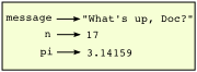
>>> message = "What's up, Doc?"
>>> n = 17
>>> pi = 3.14159
This example makes three assignments. The first assigns the string value "What's up, Doc?" to a variable named message. The second gives the integer 17 to n, and the third assigns the floating-point number 3.14159 to a variable called pi.
The assignment token, =, should not be confused with equals, which uses the token ==. The assignment statement binds a name, on the left-hand side of the operator, to a value, on the right-hand side. This is why you will get an error if you enter:
>>> 17 = n
File "<interactive input>", line 1
SyntaxError: can't assign to literal
Tip
When reading or writing code, say to yourself "n is assigned 17" or "n gets the value 17". Don't say "n equals 17".
A common way to represent variables on paper is to write the name with an arrow pointing to the variable's value. This kind of figure is called a state snapshot because it shows what state each of the variables is in at a particular instant in time. (Think of it as the variable's state of mind). This diagram shows the result of executing the assignment statements:
If you ask the interpreter to evaluate a variable, it will produce the value that is currently linked to the variable:
>>> message
'What's up, Doc?'
>>> n
17
>>> pi
3.14159
We use variables in a program to "remember" things, perhaps the current score at the football game. But variables are variable. This means they can change over time, just like the scoreboard at a football game. You can assign a value to a variable, and later assign a different value to the same variable. (This is different from maths. In maths, if you give `x` the value 3, it cannot change to link to a different value half-way through your calculations!)
>>> day = "Thursday"
>>> day
'Thursday'
>>> day = "Friday"
>>> day
'Friday'
>>> day = 21
>>> day
21
You'll notice we changed the value of day three times, and on the third assignment we even made it refer to a value that was of a different type.
A great deal of programming is about having the computer remember things, e.g. The number of missed calls on your phone, and then arranging to update or change the variable when you miss another call.
Variable names and keywords
Variable names can be arbitrarily long. They can contain both letters and digits, but they have to begin with a letter or an underscore. Although it is legal to use uppercase letters, by convention we don't. If you do, remember that case matters. Bruce and bruce are different variables.
The underscore character ( _) can appear in a name. It is often used in names with multiple words, such as my_name or price_of_tea_in_china.
There are some situations in which names beginning with an underscore have special meaning, so a safe rule for beginners is to start all names with a letter.
If you give a variable an illegal name, you get a syntax error:
>>> 76trombones = "big parade"
SyntaxError: invalid syntax
>>> more$ = 1000000
SyntaxError: invalid syntax
>>> class = "Computer Science 101"
SyntaxError: invalid syntax
76trombones is illegal because it does not begin with a letter. more$ is illegal because it contains an illegal character, the dollar sign. But what's wrong with class?
It turns out that class is one of the Python keywords. Keywords define the language's syntax rules and structure, and they cannot be used as variable names.
Python has thirty-something keywords (and every now and again improvements to Python introduce or eliminate one or two):
| and | as | assert | break | class | continue |
| def | del | elif | else | except | exec |
| finally | for | from | global | if | import |
| in | is | lambda | nonlocal | not | or |
| pass | raise | return | try | while | with |
| yield | True | False | None |
You might want to keep this list handy. If the interpreter complains about one of your variable names and you don't know why, see if it is on this list.
Programmers generally choose names for their variables that are meaningful to the human readers of the program --- they help the programmer document, or remember, what the variable is used for.
Caution!
Beginners sometimes confuse "meaningful to the human readers" with "meaningful to the computer". So they'll wrongly think that because they've called some variable average or pi, it will somehow magically calculate an average, or magically know that the variable pi should have a value like 3.14159. No! The computer doesn't understand what you intend the variable to mean.
So you'll find some instructors who deliberately don't choose meaningful names when they teach beginners --- not because we don't think it is a good habit, but because we're trying to reinforce the message that you --- the programmer --- must write the program code to calculate the average, and you must write an assignment statement to give the variable pi the value you want it to have.
Statements
A statement is an instruction that the Python interpreter can execute. We have only seen the assignment statement so far. Some other kinds of statements that we'll see shortly are while statements, for statements, if statements, and import statements. (There are other kinds too!)
When you type a statement on the command line, Python executes it. Statements don't produce any result.
Evaluating expressions
An expression is a combination of values, variables, operators, and calls to functions. If you type an expression at the Python prompt, the interpreter evaluates it and displays the result:
>>> 1 + 1
2
>>> len("hello")
5
In this example len is a built-in Python function that returns the number of characters in a string. We've previously seen the print and the type functions, so this is our third example of a function!
The evaluation of an expression produces a value, which is why expressions can appear on the right hand side of assignment statements. A value all by itself is a simple expression, and so is a variable.
>>> 17
17
>>> y = 3.14
>>> x = len("hello")
>>> x
5
>>> y
3.14
Operators and operands
Operators are special tokens that represent computations like addition, multiplication and division. The values the operator uses are called operands.
The following are all legal Python expressions whose meaning is more or less clear:
20+32 hour-1 hour*60+minute minute/60 5**2 (5+9)*(15-7)
The tokens +, -, and *, and the use of parenthesis for grouping, mean in Python what they mean in mathematics. The asterisk (*) is the token for multiplication, and ** is the token for exponentiation.
>>> 2 ** 3
8
>>> 3 ** 2
9
When a variable name appears in the place of an operand, it is replaced with its value before the operation is performed.
Addition, subtraction, multiplication, and exponentiation all do what you expect.
Example: so let us convert 645 minutes into hours:
>>> minutes = 645
>>> hours = minutes / 60
>>> hours
10.75
Oops! In Python 3, the division operator / always yields a floating point result. What we might have wanted to know was how many whole hours there are, and how many minutes remain. Python gives us two different flavors of the division operator. The second, called floor division uses the token //. Its result is always a whole number --- and if it has to adjust the number it always moves it to the left on the number line. So 6 // 4 yields 1, but -6 // 4 might surprise you!
>>> 7 / 4
1.75
>>> 7 // 4
1
>>> minutes = 645
>>> hours = minutes // 60
>>> hours
10
Take care that you choose the correct flavor of the division operator. If you're working with expressions where you need floating point values, use the division operator that does the division accurately.
Type converter functions
Here we'll look at three more Python functions, int, float and str, which will (attempt to) convert their arguments into types int, float and str respectively. We call these type converter functions.
The int function can take a floating point number or a string, and turn it into an int. For floating point numbers, it discards the decimal portion of the number --- a process we call truncation towards zero on the number line. Let us see this in action:
>>> int(3.14)
3
>>> int(3.9999)             # This doesn't round to the closest int!
3
>>> int(3.0)
3
>>> int(-3.999)             # Note that the result is closer to zero
-3
>>> int(minutes / 60)
10
>>> int("2345")             # Parse a string to produce an int
2345
>>> int(17)                 # It even works if arg is already an int
17
>>> int("23 bottles")
This last case doesn't look like a number --- what do we expect?
Traceback (most recent call last):
File "<interactive input>", line 1, in <module>
ValueError: invalid literal for int() with base 10: '23 bottles'
The type converter float can turn an integer, a float, or a syntactically legal string into a float:
>>> float(17)
17.0
>>> float("123.45")
123.45
The type converter str turns its argument into a string:
>>> str(17)
'17'
>>> str(123.45)
'123.45'
Order of operations
When more than one operator appears in an expression, the order of evaluation depends on the rules of precedence. Python follows the same precedence rules for its mathematical operators that mathematics does. The acronym PEMDAS is a useful way to remember the order of operations:
Parentheses have the highest precedence and can be used to force an expression to evaluate in the order you want. Since expressions in parentheses are evaluated first, 2 * (3-1) is 4, and (1+1)**(5-2) is 8. You can also use parentheses to make an expression easier to read, as in (minute * 100) / 60, even though it doesn't change the result.
Exponentiation has the next highest precedence, so 2**1+1 is 3 and not 4, and 3*1**3 is 3 and not 27.
Multiplication and both Division operators have the same precedence, which is higher than Addition and Subtraction, which also have the same precedence. So 2*3-1 yields 5 rather than 4, and 5-2*2 is 1, not 6.
Operators with the same precedence are evaluated from left-to-right. In algebra we say they are left-associative. So in the expression 6-3+2, the subtraction happens first, yielding 3. We then add 2 to get the result 5. If the operations had been evaluated from right to left, the result would have been 6-(3+2), which is 1. (The acronym PEDMAS could mislead you to thinking that division has higher precedence than multiplication, and addition is done ahead of subtraction - don't be misled. Subtraction and addition are at the same precedence, and the left-to-right rule applies.)
Due to some historical quirk, an exception to the left-to-right left-associative rule is the exponentiation operator **, so a useful hint is to always use parentheses to force exactly the order you want when exponentiation is involved:
>>> 2 ** 3 ** 2     # The right-most ** operator gets done first!
512
>>> (2 ** 3) ** 2   # Use parentheses to force the order you want!
64
The immediate mode command prompt of Python is great for exploring and experimenting with expressions like this.
Operations on strings
In general, you cannot perform mathematical operations on strings, even if the strings look like numbers. The following are illegal (assuming that message has type string):
>>> message - 1        # Error
>>> "Hello" / 123      # Error
>>> message * "Hello"  # Error
>>> "15" + 2           # Error
Interestingly, the + operator does work with strings, but for strings, the + operator represents concatenation, not addition. Concatenation means joining the two operands by linking them end-to-end. For example:
fruit = "banana"
baked_good = " nut bread"
print(fruit + baked_good)
The output of this program is banana nut bread. The space before the word nut is part of the string, and is necessary to produce the space between the concatenated strings.
The * operator also works on strings; it performs repetition. For example, 'Fun'*3 is 'FunFunFun'. One of the operands has to be a string; the other has to be an integer.
On one hand, this interpretation of + and * makes sense by analogy with addition and multiplication. Just as 4*3 is equivalent to 4+4+4, we expect "Fun"*3 to be the same as "Fun"+"Fun"+"Fun", and it is. On the other hand, there is a significant way in which string concatenation and repetition are different from integer addition and multiplication. Can you think of a property that addition and multiplication have that string concatenation and repetition do not?
Input
There is a built-in function in Python for getting input from the user:
n = input("Please enter your name: ")
A sample run of this script in PyScripter would pop up a dialog window like this:
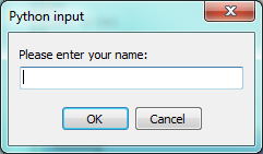
The user of the program can enter the name and click OK, and when this happens the text that has been entered is returned from the input function, and in this case assigned to the variable n.
Even if you asked the user to enter their age, you would get back a string like "17". It would be your job, as the programmer, to convert that string into a int or a float, using the int or float converter functions we saw earlier.
Composition
So far, we have looked at the elements of a program --- variables, expressions, statements, and function calls --- in isolation, without talking about how to combine them.
One of the most useful features of programming languages is their ability to take small building blocks and compose them into larger chunks.
For example, we know how to get the user to enter some input, we know how to convert the string we get into a float, we know how to write a complex expression, and we know how to print values. Let's put these together in a small four-step program that asks the user to input a value for the radius of a circle, and then computes the area of the circle from the formula.

Firstly, we'll do the four steps one at a time:
response = input("What is your radius? ")
r = float(response)
area = 3.14159 * r**2
print("The area is ", area)
Now let's compose the first two lines into a single line of code, and compose the second two lines into another line of code.
r = float( input("What is your radius? ") )
print("The area is ", 3.14159 * r**2)
If we really wanted to be tricky, we could write it all in one statement:
print("The area is ", 3.14159*float(input("What is your radius?"))**2)
Such compact code may not be most understandable for humans, but it does illustrate how we can compose bigger chunks from our building blocks.
If you're ever in doubt about whether to compose code or fragment it into smaller steps, try to make it as simple as you can for the human to follow. My choice would be the first case above, with four separate steps.
The modulus operator
The modulus operator works on integers (and integer expressions) and gives the remainder when the first number is divided by the second. In Python, the modulus operator is a percent sign (%). The syntax is the same as for other operators. It has the same precedence as the multiplication operator.
>>> q = 7 // 3     # This is integer division operator
>>> print(q)
2
>>> r  = 7 % 3
>>> print(r)
1
So 7 divided by 3 is 2 with a remainder of 1.
The modulus operator turns out to be surprisingly useful. For example, you can check whether one number is divisible by another---if x % y is zero, then x is divisible by y.
Also, you can extract the right-most digit or digits from a number. For example, x % 10 yields the right-most digit of x (in base 10). Similarly x % 100 yields the last two digits.
It is also extremely useful for doing conversions, say from seconds, to hours, minutes and seconds. So let's write a program to ask the user to enter some seconds, and we'll convert them into hours, minutes, and remaining seconds.
total_secs = int(input("How many seconds, in total?"))
hours = total_secs // 3600
secs_still_remaining = total_secs % 3600
minutes =  secs_still_remaining // 60
secs_finally_remaining = secs_still_remaining  % 60

print("Hrs=", hours, "  mins=", minutes,
                         "secs=", secs_finally_remaining)
Glossary
- assignment statement
A statement that assigns a value to a name (variable). To the left of the assignment operator, =, is a name. To the right of the assignment token is an expression which is evaluated by the Python interpreter and then assigned to the name. The difference between the left and right hand sides of the assignment statement is often confusing to new programmers. In the following assignment:
n = n + 1n plays a very different role on each side of the =. On the right it is a value and makes up part of the expression which will be evaluated by the Python interpreter before assigning it to the name on the left.
- assignment token
- = is Python's assignment token. Do not confuse it with equals, which is an operator for comparing values.
- composition
- The ability to combine simple expressions and statements into compound statements and expressions in order to represent complex computations concisely.
- concatenate
- To join two strings end-to-end.
- data type
- A set of values. The type of a value determines how it can be used in expressions. So far, the types you have seen are integers (int), floating-point numbers (float), and strings (str).
- evaluate
- To simplify an expression by performing the operations in order to yield a single value.
- expression
- A combination of variables, operators, and values that represents a single result value.
- float
- A Python data type which stores floating-point numbers. Floating-point numbers are stored internally in two parts: a base and an exponent. When printed in the standard format, they look like decimal numbers. Beware of rounding errors when you use floats, and remember that they are only approximate values.
- floor division
- An operator (denoted by the token //) that divides one number by another and yields an integer, or, if the result is not already an integer, it yields the next smallest integer.
- int
- A Python data type that holds positive and negative whole numbers.
- keyword
- A reserved word that is used by the compiler to parse program; you cannot use keywords like if, def, and while as variable names.
- modulus operator
- An operator, denoted with a percent sign ( %), that works on integers and yields the remainder when one number is divided by another.
- operand
- One of the values on which an operator operates.
- operator
- A special symbol that represents a simple computation like addition, multiplication, or string concatenation.
- rules of precedence
- The set of rules governing the order in which expressions involving multiple operators and operands are evaluated.
- state snapshot
- A graphical representation of a set of variables and the values to which they refer, taken at a particular instant during the program's execution.
- statement
- An instruction that the Python interpreter can execute. So far we have only seen the assignment statement, but we will soon meet the import statement and the for statement.
- str
- A Python data type that holds a string of characters.
- value
- A number or string (or other things to be named later) that can be stored in a variable or computed in an expression.
- variable
- A name that refers to a value.
- variable name
- A name given to a variable. Variable names in Python consist of a sequence of letters (a..z, A..Z, and _) and digits (0..9) that begins with a letter. In best programming practice, variable names should be chosen so that they describe their use in the program, making the program self documenting.
References
| [ThinkCS] | How To Think Like a Computer Scientist --- Learning with Python 3 |
Hello, little turtles!
Source: this section is heavily based on Chapter 3 of [ThinkCS].
There are many modules in Python that provide very powerful features that we can use in our own programs. Some of these can send email, or fetch web pages. The one we'll look at in this chapter allows us to create turtles and get them to draw shapes and patterns.
The turtles are fun, but the real purpose of the chapter is to teach ourselves a little more Python, and to develop our theme of computational thinking, or thinking like a computer scientist. Most of the Python covered here will be explored in more depth later.
Our first turtle program
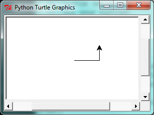
Let's write a couple of lines of Python program to create a new turtle and start drawing a rectangle. (We'll call the variable that refers to our first turtle alex, but we can choose another name if we follow the naming rules from the previous chapter).
import turtle             # Allows us to use turtles
wn = turtle.Screen()      # Creates a playground for turtles
alex = turtle.Turtle()    # Create a turtle, assign to alex

alex.forward(50)          # Tell alex to move forward by 50 units
alex.left(90)             # Tell alex to turn by 90 degrees
alex.forward(30)          # Complete the second side of a rectangle

wn.mainloop()             # Wait for user to close window
When we run this program, a new window pops up:
Here are a couple of things we'll need to understand about this program.
The first line tells Python to load a module named turtle. That module brings us two new types that we can use: the Turtle type, and the Screen type. The dot notation turtle.Turtle means "The Turtle type that is defined within the turtle module". (Remember that Python is case sensitive, so the module name, with a lowercase t, is different from the type Turtle.)
We then create and open what it calls a screen (we would prefer to call it a window), which we assign to variable wn. Every window contains a canvas, which is the area inside the window on which we can draw.
In line 3 we create a turtle. The variable alex is made to refer to this turtle.
So these first three lines have set things up, we're ready to get our turtle to draw on our canvas.
In lines 5-7, we instruct the object alex to move, and to turn. We do this by invoking, or activating, alex's methods --- these are the instructions that all turtles know how to respond to.
The last line plays a part too: the wn variable refers to the window shown above. When we invoke its mainloop method, it enters a state where it waits for events (like keypresses, or mouse movement and clicks). The program will terminate when the user closes the window.
An object can have various methods --- things it can do --- and it can also have attributes --- (sometimes called properties). For example, each turtle has a color attribute. The method invocation alex.color("red") will make alex red, and drawing will be red too. (Note the word color is spelled the American way!)
The color of the turtle, the width of its pen, the position of the turtle within the window, which way it is facing, and so on are all part of its current state. Similarly, the window object has a background color, and some text in the title bar, and a size and position on the screen. These are all part of the state of the window object.
Quite a number of methods exist that allow us to modify the turtle and the window objects. We'll just show a couple. In this program we've only commented those lines that are different from the previous example (and we've used a different variable name for this turtle):
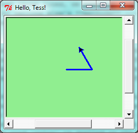
import turtle
wn = turtle.Screen()
wn.bgcolor("lightgreen")      # Set the window background color
wn.title("Hello, Tess!")      # Set the window title

tess = turtle.Turtle()
tess.color("blue")            # Tell tess to change her color
tess.pensize(3)               # Tell tess to set her pen width

tess.forward(50)
tess.left(120)
tess.forward(50)

wn.mainloop()
When we run this program, a new window pops up, and will remain on the screen until we close it.
Extend this program ...
- Modify this program so that before it creates the window, it prompts the user to enter the desired background color. It should store the user's responses in a variable, and modify the color of the window according to the user's wishes. (Hint: you can find a list of permitted color names at http://www.tcl.tk/man/tcl8.4/TkCmd/colors.htm. It includes some quite unusual ones, like "peach puff" and "HotPink".)
- Do similar changes to allow the user, at runtime, to set tess' color.
- Do the same for the width of tess' pen. Hint: your dialog with the user will return a string, but tess' pensize method expects its argument to be an int. So you'll need to convert the string to an int before you pass it to pensize.
Instances --- a herd of turtles
Just like we can have many different integers in a program, we can have many turtles. Each of them is called an instance. Each instance has its own attributes and methods --- so alex might draw with a thin black pen and be at some position, while tess might be going in her own direction with a fat pink pen.
import turtle
wn = turtle.Screen()         # Set up the window and its attributes
wn.bgcolor("lightgreen")
wn.title("Tess & Alex")

tess = turtle.Turtle()       # Create tess and set some attributes
tess.color("hotpink")
tess.pensize(5)

alex = turtle.Turtle()       # Create alex

tess.forward(80)             # Make tess draw equilateral triangle
tess.left(120)
tess.forward(80)
tess.left(120)
tess.forward(80)
tess.left(120)               # Complete the triangle

tess.right(180)              # Turn tess around
tess.forward(80)             # Move her away from the origin

alex.forward(50)             # Make alex draw a square
alex.left(90)
alex.forward(50)
alex.left(90)
alex.forward(50)
alex.left(90)
alex.forward(50)
alex.left(90)

wn.mainloop()
Here is what happens when alex completes his rectangle, and tess completes her triangle:
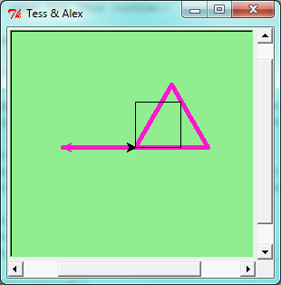
Here are some How to think like a computer scientist observations:
- There are 360 degrees in a full circle. If we add up all the turns that a turtle makes, no matter what steps occurred between the turns, we can easily figure out if they add up to some multiple of 360. This should convince us that alex is facing in exactly the same direction as he was when he was first created. (Geometry conventions have 0 degrees facing East, and that is the case here too!)
- We could have left out the last turn for alex, but that would not have been as satisfying. If we're asked to draw a closed shape like a square or a rectangle, it is a good idea to complete all the turns and to leave the turtle back where it started, facing the same direction as it started in. This makes reasoning about the program and composing chunks of code into bigger programs easier for us humans!
- We did the same with tess: she drew her triangle, and turned through a full 360 degrees. Then we turned her around and moved her aside. Even the blank line 18 is a hint about how the programmer's mental chunking is working: in big terms, tess' movements were chunked as "draw the triangle" (lines 12-17) and then "move away from the origin" (lines 19 and 20).
- One of the key uses for comments is to record our mental chunking, and big ideas. They're not always explicit in the code.
- And, uh-huh, two turtles may not be enough for a herd. But the important idea is that the turtle module gives us a kind of factory that lets us create as many turtles as we need. Each instance has its own state and behaviour.
The for loop
When we drew the square, it was quite tedious. We had to explicitly repeat the steps of moving and turning four times. If we were drawing a hexagon, or an octogon, or a polygon with 42 sides, it would have been worse.
So a basic building block of all programs is to be able to repeat some code, over and over again.
Python's for loop solves this for us. Let's say we have some friends, and we'd like to send them each an email inviting them to our party. We don't quite know how to send email yet, so for the moment we'll just print a message for each friend:
for f in ["Joe","Zoe","Brad","Angelina","Zuki","Thandi","Paris"]:
    invite = "Hi " + f + ".  Please come to my party on Saturday!"
    print(invite)
# more code can follow here ...
When we run this, the output looks like this:
Hi Joe.  Please come to my party on Saturday!
Hi Zoe.  Please come to my party on Saturday!
Hi Brad.  Please come to my party on Saturday!
Hi Angelina.  Please come to my party on Saturday!
Hi Zuki.  Please come to my party on Saturday!
Hi Thandi.  Please come to my party on Saturday!
Hi Paris.  Please come to my party on Saturday!
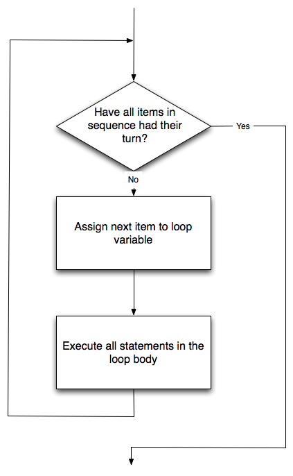
- The variable f in the for statement at line 1 is called the loop variable. We could have chosen any other variable name instead.
- Lines 2 and 3 are the loop body. The loop body is always indented. The indentation determines exactly what statements are "in the body of the loop".
- On each iteration or pass of the loop, first a check is done to see if there are still more items to be processed. If there are none left (this is called the terminating condition of the loop), the loop has finished. Program execution continues at the next statement after the loop body, (e.g. in this case the next statement below the comment in line 4).
- If there are items still to be processed, the loop variable is updated to refer to the next item in the list. This means, in this case, that the loop body is executed here 7 times, and each time f will refer to a different friend.
- At the end of each execution of the body of the loop, Python returns to the for statement, to see if there are more items to be handled, and to assign the next one to f.
Flow of Execution of the for loop
As a program executes, the interpreter always keeps track of which statement is about to be executed. We call this the control flow, of the flow of execution of the program. When humans execute programs, they often use their finger to point to each statement in turn. So we could think of control flow as "Python's moving finger".
Control flow until now has been strictly top to bottom, one statement at a time. The for loop changes this.
Flowchart of a for loop
Control flow is often easy to visualize and understand if we draw a flowchart. This shows the exact steps and logic of how the for statement executes.
The loop simplifies our turtle program
To draw a square we'd like to do the same thing four times --- move the turtle, and turn. We previously used 8 lines to have alex draw the four sides of a square. This does exactly the same, but using just three lines:
for i in [0,1,2,3]:
    alex.forward(50)
    alex.left(90)
Some observations:
While "saving some lines of code" might be convenient, it is not the big deal here. What is much more important is that we've found a "repeating pattern" of statements, and reorganized our program to repeat the pattern. Finding the chunks and somehow getting our programs arranged around those chunks is a vital skill in computational thinking.
The values [0,1,2,3] were provided to make the loop body execute 4 times. We could have used any four values, but these are the conventional ones to use. In fact, they are so popular that Python gives us special built-in range objects:
for i in range(4):
    # Executes the body with i = 0, then 1, then 2, then 3
for x in range(10):
    # Sets x to each of ... [0, 1, 2, 3, 4, 5, 6, 7, 8, 9]
Computer scientists like to count from 0!
range can deliver a sequence of values to the loop variable in the for loop. They start at 0, and in these cases do not include the 4 or the 10.
Our little trick earlier to make sure that alex did the final turn to complete 360 degrees has paid off: if we had not done that, then we would not have been able to use a loop for the fourth side of the square. It would have become a "special case", different from the other sides. When possible, we'd much prefer to make our code fit a general pattern, rather than have to create a special case.
So to repeat something four times, a good Python programmer would do this:
for i in range(4):
    alex.forward(50)
    alex.left(90)
By now you should be able to see how to change our previous program so that tess can also use a for loop to draw her equilateral triangle.
But now, what would happen if we made this change?
for c in ["yellow", "red", "purple", "blue"]:
    alex.color(c)
    alex.forward(50)
    alex.left(90)
A variable can also be assigned a value that is a list. So lists can also be used in more general situations, not only in the for loop. The code above could be rewritten like this:
# Assign a list to a variable
clrs = ["yellow", "red", "purple", "blue"]
for c in clrs:
    alex.color(c)
    alex.forward(50)
    alex.left(90)
A few more turtle methods and tricks
Turtle methods can use negative angles or distances. So tess.forward(-100) will move tess backwards, and tess.left(-30) turns her to the right. Additionally, because there are 360 degrees in a circle, turning 30 to the left will get tess facing in the same direction as turning 330 to the right! (The on-screen animation will differ, though --- you will be able to tell if tess is turning clockwise or counter-clockwise!)
This suggests that we don't need both a left and a right turn method --- we could be minimalists, and just have one method. There is also a backward method. (If you are very nerdy, you might enjoy saying alex.backward(-100) to move alex forward!)
Part of thinking like a scientist is to understand more of the structure and rich relationships in our field. So revising a few basic facts about geometry and number lines, and spotting the relationships between left, right, backward, forward, negative and positive distances or angles values is a good start if we're going to play with turtles.
A turtle's pen can be picked up or put down. This allows us to move a turtle to a different place without drawing a line. The methods are
alex.penup()
alex.forward(100)     # This moves alex, but no line is drawn
alex.pendown()
Every turtle can have its own shape. The ones available "out of the box" are arrow, blank, circle, classic, square, triangle, turtle.
alex.shape("turtle")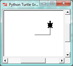
We can speed up or slow down the turtle's animation speed. (Animation controls how quickly the turtle turns and moves forward). Speed settings can be set between 1 (slowest) to 10 (fastest). But if we set the speed to 0, it has a special meaning --- turn off animation and go as fast as possible.
alex.speed(10)
A turtle can "stamp" its footprint onto the canvas, and this will remain after the turtle has moved somewhere else. Stamping works, even when the pen is up.
Let's do an example that shows off some of these new features:
import turtle
wn = turtle.Screen()
wn.bgcolor("lightgreen")
tess = turtle.Turtle()
tess.shape("turtle")
tess.color("blue")

tess.penup()                # This is new
size = 20
for i in range(30):
   tess.stamp()             # Leave an impression on the canvas
   size = size + 3          # Increase the size on every iteration
   tess.forward(size)       # Move tess along
   tess.right(24)           #  ...  and turn her

wn.mainloop()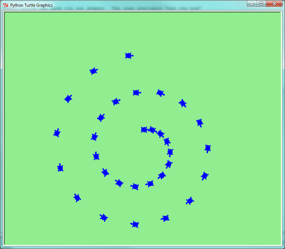
Be careful now! How many times was the body of the loop executed? How many turtle images do we see on the screen? All except one of the shapes we see on the screen here are footprints created by stamp. But the program still only has one turtle instance --- can you figure out which one here is the real tess? (Hint: if you're not sure, write a new line of code after the for loop to change tess' color, or to put her pen down and draw a line, or to change her shape, etc.)
Glossary
- attribute
- Some state or value that belongs to a particular object. For example, tess has a color.
- canvas
- A surface within a window where drawing takes place.
- control flow
- See flow of execution in the next chapter.
- for loop
- A statement in Python for convenient repetition of statements in the body of the loop.
- loop body
- Any number of statements nested inside a loop. The nesting is indicated by the fact that the statements are indented under the for loop statement.
- loop variable
- A variable used as part of a for loop. It is assigned a different value on each iteration of the loop.
- instance
- An object of a certain type, or class. tess and alex are different instances of the class Turtle.
- method
- A function that is attached to an object. Invoking or activating the method causes the object to respond in some way, e.g. forward is the method when we say tess.forward(100).
- invoke
- An object has methods. We use the verb invoke to mean activate the method. Invoking a method is done by putting parentheses after the method name, with some possible arguments. So tess.forward() is an invocation of the forward method.
- module
- A file containing Python definitions and statements intended for use in other Python programs. The contents of a module are made available to the other program by using the import statement.
- object
- A "thing" to which a variable can refer. This could be a screen window, or one of the turtles we have created.
- range
- A built-in function in Python for generating sequences of integers. It is especially useful when we need to write a for loop that executes a fixed number of times.
- terminating condition
- A condition that occurs which causes a loop to stop repeating its body. In the for loops we saw in this chapter, the terminating condition has been when there are no more elements to assign to the loop variable.
References
| [ThinkCS] | How To Think Like a Computer Scientist --- Learning with Python 3 |
Functions
Source: this section is heavily based on Chapter 4 of [ThinkCS].
Functions
In Python, a function is a named sequence of statements that belong together. Their primary purpose is to help us organize programs into chunks that match how we think about the problem.
The syntax for a function definition is:
def NAME( PARAMETERS ):
    STATEMENTS
We can make up any names we want for the functions we create, except that we can't use a name that is a Python keyword, and the names must follow the rules for legal identifiers.
There can be any number of statements inside the function, but they have to be indented from the def. In the examples in this book, we will use the standard indentation of four spaces. Function definitions are the second of several compound statements we will see, all of which have the same pattern:
- A header line which begins with a keyword and ends with a colon.
- A body consisting of one or more Python statements, each indented the same amount --- the Python style guide recommends 4 spaces --- from the header line.
We've already seen the for loop which follows this pattern.
So looking again at the function definition, the keyword in the header is def, which is followed by the name of the function and some parameters enclosed in parentheses. The parameter list may be empty, or it may contain any number of parameters separated from one another by commas. In either case, the parentheses are required. The parameters specifies what information, if any, we have to provide in order to use the new function.
Suppose we're working with turtles, and a common operation we need is to draw squares. "Draw a square" is an abstraction, or a mental chunk, of a number of smaller steps. So let's write a function to capture the pattern of this "building block":
import turtle

def draw_square(t, sz):
    """Make turtle t draw a square of sz."""
    for i in range(4):
        t.forward(sz)
        t.left(90)


wn = turtle.Screen()        # Set up the window and its attributes
wn.bgcolor("lightgreen")
wn.title("Alex meets a function")

alex = turtle.Turtle()      # Create alex
draw_square(alex, 50)       # Call the function to draw the square
wn.mainloop()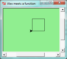
This function is named draw_square. It has two parameters: one to tell the function which turtle to move around, and the other to tell it the size of the square we want drawn. Make sure you know where the body of the function ends --- it depends on the indentation, and the blank lines don't count for this purpose!
Docstrings for documentation
If the first thing after the function header is a string, it is treated as a docstring and gets special treatment in Python and in some programming tools. For example, when we type a built-in function name with an unclosed parenthesis in PyScripter, a tooltip pops up, telling us what arguments the function takes, and it shows us any other text contained in the docstring.
Docstrings are the key way to document our functions in Python and the documentation part is important. Because whoever calls our function shouldn't have to need to know what is going on in the function or how it works; they just need to know what arguments our function takes, what it does, and what the expected result is. Enough to be able to use the function without having to look underneath. This goes back to the concept of abstraction of which we'll talk more about.
Docstrings are usually formed using triple-quoted strings as they allow us to easily expand the docstring later on should we want to write more than a one-liner.
Just to differentiate from comments, a string at the start of a function (a docstring) is retrievable by Python tools at runtime. By contrast, comments are completely eliminated when the program is parsed.
Defining a new function does not make the function run. To do that we need a function call. We've already seen how to call some built-in functions like print, range and int. Function calls contain the name of the function being executed followed by a list of values, called arguments, which are assigned to the parameters in the function definition. So in the second last line of the program, we call the function, and pass alex as the turtle to be manipulated, and 50 as the size of the square we want. While the function is executing, then, the variable sz refers to the value 50, and the variable t refers to the same turtle instance that the variable alex refers to.
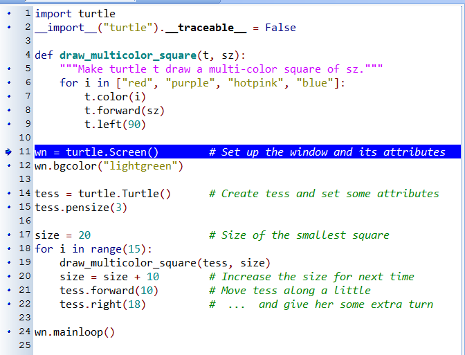
Once we've defined a function, we can call it as often as we like, and its statements will be executed each time we call it. And we could use it to get any of our turtles to draw a square. In the next example, we've changed the draw_square function a little, and we get tess to draw 15 squares, with some variations.
import turtle

def draw_multicolor_square(t, sz):
    """Make turtle t draw a multi-color square of sz."""
    for i in ["red", "purple", "hotpink", "blue"]:
        t.color(i)
        t.forward(sz)
        t.left(90)

wn = turtle.Screen()        # Set up the window and its attributes
wn.bgcolor("lightgreen")

tess = turtle.Turtle()      # Create tess and set some attributes
tess.pensize(3)

size = 20                   # Size of the smallest square
for i in range(15):
    draw_multicolor_square(tess, size)
    size = size + 10        # Increase the size for next time
    tess.forward(10)        # Move tess along a little
    tess.right(18)          #    and give her some turn

wn.mainloop()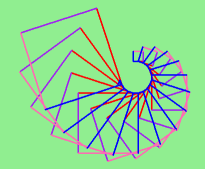
Functions can call other functions
Let's assume now we want a function to draw a rectangle. We need to be able to call the function with different arguments for width and height. And, unlike the case of the square, we cannot repeat the same thing 4 times, because the four sides are not equal.
So we eventually come up with this rather nice code that can draw a rectangle.
def draw_rectangle(t, w, h):
    """Get turtle t to draw a rectangle of width w and height h."""
    for i in range(2):
        t.forward(w)
        t.left(90)
        t.forward(h)
        t.left(90)
The parameter names are deliberately chosen as single letters to ensure they're not misunderstood. In real programs, once we've had more experience, we will insist on better variable names than this. But the point is that the program doesn't "understand" that we're drawing a rectangle, or that the parameters represent the width and the height. Concepts like rectangle, width, and height are the meaning we humans have, not concepts that the program or the computer understands.
Thinking like a scientist involves looking for patterns and relationships. In the code above, we've done that to some extent. We did not just draw four sides. Instead, we spotted that we could draw the rectangle as two halves, and used a loop to repeat that pattern twice.
But now we might spot that a square is a special kind of rectangle. We already have a function that draws a rectangle, so we can use that to draw our square.
def draw_square(tx, sz):        # A new version of draw_square
    draw_rectangle(tx, sz, sz)
There are some points worth noting here:
- Functions can call other functions.
- Rewriting draw_square like this captures the relationship that we've spotted between squares and rectangles.
- A caller of this function might say draw_square(tess, 50). The parameters of this function, tx and sz, are assigned the values of the tess object, and the int 50 respectively.
- In the body of the function they are just like any other variable.
- When the call is made to draw_rectangle, the values in variables tx and sz are fetched first, then the call happens. So as we enter the top of function draw_rectangle, its variable t is assigned the tess object, and w and h in that function are both given the value 50.
So far, it may not be clear why it is worth the trouble to create all of these new functions. Actually, there are a lot of reasons, but this example demonstrates two:
- Creating a new function gives us an opportunity to name a group of statements. Functions can simplify a program by hiding a complex computation behind a single command. The function (including its name) can capture our mental chunking, or abstraction, of the problem.
- Creating a new function can make a program smaller by eliminating repetitive code.
As we might expect, we have to create a function before we can execute it. In other words, the function definition has to be executed before the function is called.
Flow of execution
In order to ensure that a function is defined before its first use, we have to know the order in which statements are executed, which is called the flow of execution. We've already talked about this a little in the previous chapter.
Execution always begins at the first statement of the program. Statements are executed one at a time, in order from top to bottom.
Function definitions do not alter the flow of execution of the program, but remember that statements inside the function are not executed until the function is called. Although it is not common, we can define one function inside another. In this case, the inner definition isn't executed until the outer function is called.
Function calls are like a detour in the flow of execution. Instead of going to the next statement, the flow jumps to the first line of the called function, executes all the statements there, and then comes back to pick up where it left off.
That sounds simple enough, until we remember that one function can call another. While in the middle of one function, the program might have to execute the statements in another function. But while executing that new function, the program might have to execute yet another function!
Fortunately, Python is adept at keeping track of where it is, so each time a function completes, the program picks up where it left off in the function that called it. When it gets to the end of the program, it terminates.
What's the moral of this sordid tale? When we read a program, don't read from top to bottom. Instead, follow the flow of execution.
Watch the flow of execution in action
In PyScripter, we can watch the flow of execution by "single-stepping" through any program. PyScripter will highlight each line of code just before it is about to be executed.
PyScripter also lets us hover the mouse over any variable in the program, and it will pop up the current value of that variable. So this makes it easy to inspect the "state snapshot" of the program --- the current values that are assigned to the program's variables.
This is a powerful mechanism for building a deep and thorough understanding of what is happening at each step of the way. Learn to use the single-stepping feature well, and be mentally proactive: as you work through the code, challenge yourself before each step: "What changes will this line make to any variables in the program?" and "Where will flow of execution go next?"
Let us go back and see how this works with the program above that draws 15 multicolor squares. First, we're going to add one line of magic below the import statement --- not strictly necessary, but it will make our lives much simpler, because it prevents stepping into the module containing the turtle code.
import turtle
__import__("turtle").__traceable__ = False
Now we're ready to begin. Put the mouse cursor on the line of the program where we create the turtle screen, and press the F4 key. This will run the Python program up to, but not including, the line where we have the cursor. Our program will "break" now, and provide a highlight on the next line to be executed, something like this:
At this point we can press the F7 key (step into) repeatedly to single step through the code. Observe as we execute lines 10, 11, 12, ... how the turtle window gets created, how its canvas color is changed, how the title gets changed, how the turtle is created on the canvas, and then how the flow of execution gets into the loop, and from there into the function, and into the function's loop, and then repeatedly through the body of that loop.
While we do this, we can also hover our mouse over some of the variables in the program, and confirm that their values match our conceptual model of what is happening.
After a few loops, when we're about to execute line 20 and we're starting to get bored, we can use the key F8 to "step over" the function we are calling. This executes all the statements in the function, but without having to step through each one. We always have the choice to either "go for the detail", or to "take the high-level view" and execute the function as a single chunk.
There are some other options, including one that allow us to resume execution without further stepping. Find them under the Run menu of PyScripter.
Functions that require arguments
Most functions require arguments: the arguments provide for generalization. For example, if we want to find the absolute value of a number, we have to indicate what the number is. Python has a built-in function for computing the absolute value:
>>> abs(5)
5
>>> abs(-5)
5
In this example, the arguments to the abs function are 5 and -5.
Some functions take more than one argument. For example the built-in function pow takes two arguments, the base and the exponent. Inside the function, the values that are passed get assigned to variables called parameters.
>>> pow(2, 3)
8
>>> pow(7, 4)
2401
Another built-in function that takes more than one argument is max.
>>> max(7, 11)
11
>>> max(4, 1, 17, 2, 12)
17
>>> max(3 * 11, 5**3, 512 - 9, 1024**0)
503
max can be passed any number of arguments, separated by commas, and will return the largest value passed. The arguments can be either simple values or expressions. In the last example, 503 is returned, since it is larger than 33, 125, and 1.
Functions that return values
All the functions in the previous section return values. Furthermore, functions like range, int, abs all return values that can be used to build more complex expressions.
So an important difference between these functions and one like draw_square is that draw_square was not executed because we wanted it to compute a value --- on the contrary, we wrote draw_square because we wanted it to execute a sequence of steps that caused the turtle to draw.
A function that returns a value is called a fruitful function in this book. The opposite of a fruitful function is void function --- one that is not executed for its resulting value, but is executed because it does something useful. (Languages like Java, C#, C and C++ use the term "void function", other languages like Pascal call it a procedure.) Even though void functions are not executed for their resulting value, Python always wants to return something. So if the programmer doesn't arrange to return a value, Python will automatically return the value None.
How do we write our own fruitful function? In the exercises at the end of chapter 2 we saw the standard formula for compound interest, which we'll now write as a fruitful function:
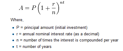 def final_amt(p, r, n, t): """ Apply the compound interest formula to p to produce the final amount. """ a = p * (1 + r/n) ** (n*t) return a # This is new, and makes the function fruitful. # now that we have the function above, let us call it. toInvest = float(input("How much do you want to invest?")) fnl = final_amt(toInvest, 0.08, 12, 5) print("At the end of the period you'll have", fnl)
The return statement is followed an expression (a in this case). This expression will be evaluated and returned to the caller as the "fruit" of calling this function.
We prompted the user for the principal amount. The type of toInvest is a string, but we need a number before we can work with it. Because it is money, and could have decimal places, we've used the float type converter function to parse the string and return a float.
Notice how we entered the arguments for 8% interest, compounded 12 times per year, for 5 years.
When we run this, we get the output
At the end of the period you'll have 14898.457083
This is a bit messy with all these decimal places, but remember that Python doesn't understand that we're working with money: it just does the calculation to the best of its ability, without rounding. Later we'll see how to format the string that is printed in such a way that it does get nicely rounded to two decimal places before printing.
The line toInvest = float(input("How much do you want to invest?")) also shows yet another example of composition --- we can call a function like float, and its arguments can be the results of other function calls (like input) that we've called along the way.
Notice something else very important here. The name of the variable we pass as an argument --- toInvest --- has nothing to do with the name of the parameter --- p. It is as if p = toInvest is executed when final_amt is called. It doesn't matter what the value was named in the caller, in final_amt its name is p.
These short variable names are getting quite tricky, so perhaps we'd prefer one of these versions instead:
def final_amt_v2(principalAmount, nominalPercentageRate,
                                    numTimesPerYear, years):
    a = principalAmount * (1 + nominalPercentageRate /
                         numTimesPerYear) ** (numTimesPerYear*years)
    return a

def final_amt_v3(amt, rate, compounded, years):
    a = amt * (1 + rate/compounded) ** (componded*years)
    return a
They all do the same thing. Use your judgement to write code that can be best understood by other humans! Short variable names are more economical and sometimes make code easier to read: E = mc2 would not be nearly so memorable if Einstein had used longer variable names! If you do prefer short names, make sure you also have some comments to enlighten the reader about what the variables are used for.
Variables and parameters are local
When we create a local variable inside a function, it only exists inside the function, and we cannot use it outside. For example, consider again this function:
def final_amt(p, r, n, t):
    a = p * (1 + r/n) ** (n*t)
    return a
If we try to use a, outside the function, we'll get an error:
>>> a
NameError: name 'a' is not defined
The variable a is local to final_amt, and is not visible outside the function.
Additionally, a only exists while the function is being executed --- we call this its lifetime. When the execution of the function terminates, the local variables are destroyed.
Parameters are also local, and act like local variables. For example, the lifetimes of p, r, n, t begin when final_amt is called, and the lifetime ends when the function completes its execution.
So it is not possible for a function to set some local variable to a value, complete its execution, and then when it is called again next time, recover the local variable. Each call of the function creates new local variables, and their lifetimes expire when the function returns to the caller.
Turtles Revisited
Now that we have fruitful functions, we can focus our attention on reorganizing our code so that it fits more nicely into our mental chunks. This process of rearrangement is called refactoring the code.
Two things we're always going to want to do when working with turtles is to create the window for the turtle, and to create one or more turtles. We could write some functions to make these tasks easier in future:
def make_window(colr, ttle):
    """
      Set up the window with the given background color and title.
      Returns the new window.
    """
    w = turtle.Screen()
    w.bgcolor(colr)
    w.title(ttle)
    return w


def make_turtle(colr, sz):
    """
      Set up a turtle with the given color and pensize.
      Returns the new turtle.
    """
    t = turtle.Turtle()
    t.color(colr)
    t.pensize(sz)
    return t


wn = make_window("lightgreen", "Tess and Alex dancing")
tess = make_turtle("hotpink", 5)
alex = make_turtle("black", 1)
dave = make_turtle("yellow", 2)
The trick about refactoring code is to anticipate which things we are likely to want to change each time we call the function: these should become the parameters, or changeable parts, of the functions we write.
Glossary
- argument
- A value provided to a function when the function is called. This value is assigned to the corresponding parameter in the function. The argument can be the result of an expression which may involve operators, operands and calls to other fruitful functions.
- body
- The second part of a compound statement. The body consists of a sequence of statements all indented the same amount from the beginning of the header. The standard amount of indentation used within the Python community is 4 spaces.
- compound statement
A statement that consists of two parts:
- header - which begins with a keyword determining the statement type, and ends with a colon.
- body - containing one or more statements indented the same amount from the header.
The syntax of a compound statement looks like this:
keyword ... : statement statement ...- docstring
- A special string that is attached to a function as its __doc__ attribute. Tools like PyScripter can use docstrings to provide documentation or hints for the programmer. When we get to modules, classes, and methods, we'll see that docstrings can also be used there.
- flow of execution
- The order in which statements are executed during a program run.
- frame
- A box in a stack diagram that represents a function call. It contains the local variables and parameters of the function.
- function
- A named sequence of statements that performs some useful operation. Functions may or may not take parameters and may or may not produce a result.
- function call
- A statement that executes a function. It consists of the name of the function followed by a list of arguments enclosed in parentheses.
- function composition
- Using the output from one function call as the input to another.
- function definition
- A statement that creates a new function, specifying its name, parameters, and the statements it executes.
- fruitful function
- A function that returns a value when it is called.
- header line
- The first part of a compound statement. A header line begins with a keyword and ends with a colon (:)
- import statement
- A statement which permits functions and variables defined in another Python module to be brought into the environment of another script. To use the features of the turtle, we need to first import the turtle module.
- lifetime
- Variables and objects have lifetimes --- they are created at some point during program execution, and will be destroyed at some time.
- local variable
- A variable defined inside a function. A local variable can only be used inside its function. Parameters of a function are also a special kind of local variable.
- parameter
- A name used inside a function to refer to the value which was passed to it as an argument.
- refactor
- A fancy word to describe reorganizing our program code, usually to make it more understandable. Typically, we have a program that is already working, then we go back to "tidy it up". It often involves choosing better variable names, or spotting repeated patterns and moving that code into a function.
- stack diagram
- A graphical representation of a stack of functions, their variables, and the values to which they refer.
- traceback
- A list of the functions that are executing, printed when a runtime error occurs. A traceback is also commonly refered to as a stack trace, since it lists the functions in the order in which they are stored in the runtime stack.
- void function
- The opposite of a fruitful function: one that does not return a value. It is executed for the work it does, rather than for the value it returns.
References
| [ThinkCS] | How To Think Like a Computer Scientist --- Learning with Python 3 |
Conditionals
Source: this section is heavily based on Chapter 5 of [ThinkCS].
Programs get really interesting when we can test conditions and change the program behaviour depending on the outcome of the tests. That's what this chapter is about.
Boolean values and expressions
A Boolean value is either true or false. It is named after the British mathematician, George Boole, who first formulated Boolean algebra --- some rules for reasoning about and combining these values. This is the basis of all modern computer logic.
In Python, the two Boolean values are True and False (the capitalization must be exactly as shown), and the Python type is bool.
>>> type(True)
<class 'bool'>
>>> type(true)
Traceback (most recent call last):
  File "<interactive input>", line 1, in <module>
NameError: name 'true' is not defined
A Boolean expression is an expression that evaluates to produce a result which is a Boolean value. For example, the operator == tests if two values are equal. It produces (or yields) a Boolean value:
>>> 5 == (3 + 2)   # Is five equal 5 to the result of 3 + 2?
True
>>> 5 == 6
False
>>> j = "hel"
>>> j + "lo" == "hello"
True
In the first statement, the two operands evaluate to equal values, so the expression evaluates to True; in the second statement, 5 is not equal to 6, so we get False.
The == operator is one of six common comparison operators which all produce a bool result; here are all six:
x == y               # Produce True if ... x is equal to y
x != y               # ... x is not equal to y
x > y                # ... x is greater than y
x < y                # ... x is less than y
x >= y               # ... x is greater than or equal to y
x <= y               # ... x is less than or equal to y
Although these operations are probably familiar, the Python symbols are different from the mathematical symbols. A common error is to use a single equal sign (=) instead of a double equal sign (==). Remember that = is an assignment operator and == is a comparison operator. Also, there is no such thing as =< or =>.
Like any other types we've seen so far, Boolean values can be assigned to variables, printed, etc.
>>> age = 18
>>> old_enough_to_get_driving_licence = age >= 17
>>> print(old_enough_to_get_driving_licence)
True
>>> type(old_enough_to_get_driving_licence)
<class 'bool'>
Logical operators
There are three logical operators, and, or, and not, that allow us to build more complex Boolean expressions from simpler Boolean expressions. The semantics (meaning) of these operators is similar to their meaning in English. For example, x > 0 and x < 10 produces True only if x is greater than 0 and at the same time, x is less than 10.
n % 2 == 0 or n % 3 == 0 is True if either of the conditions is True, that is, if the number n is divisible by 2 or it is divisible by 3. (What do you think happens if n is divisible by both 2 and by 3 at the same time? Will the expression yield True or False? Try it in your Python interpreter.)
Finally, the not operator negates a Boolean value, so not (x > y) is True if (x > y) is False, that is, if x is less than or equal to y.
The expression on the left of the or operator is evaluated first: if the result is True, Python does not (and need not) evaluate the expression on the right --- this is called short-circuit evaluation. Similarly, for the and operator, if the expression on the left yields False, Python does not evaluate the expression on the right.
So there are no unnecessary evaluations.
Truth Tables
A truth table is a small table that allows us to list all the possible inputs, and to give the results for the logical operators. Because the and and or operators each have two operands, there are only four rows in a truth table that describes the semantics of and.
a b a and b False False False False True False True False False True True True
In a Truth Table, we sometimes use T and F as shorthand for the two Boolean values: here is the truth table describing or:
a b a or b F F F F T T T F T T T T
The third logical operator, not, only takes a single operand, so its truth table only has two rows:
a not a F T T F
Simplifying Boolean Expressions
A set of rules for simplifying and rearranging expressions is called an algebra. For example, we are all familiar with school algebra rules, such as:
n * 0 == 0
Here we see a different algebra --- the Boolean algebra --- which provides rules for working with Boolean values.
First, the and operator:
x and False == False
False and x == False
y and x == x and y
x and True == x
True and x == x
x and x == x
Here are some corresponding rules for the or operator:
x or False == x
False or x == x
y or x == x or y
x or True == True
True or x == True
x or x == x
Two not operators cancel each other:
not (not x) == x
Conditional execution
In order to write useful programs, we almost always need the ability to check conditions and change the behavior of the program accordingly. Conditional statements give us this ability. The simplest form is the if statement:
if x % 2 == 0:
    print(x, " is even.")
    print("Did you know that 2 is the only even number that is prime?")
else:
    print(x, " is odd.")
    print("Did you know that multiplying two odd numbers " +
                                         "always gives an odd result?")
The Boolean expression after the if statement is called the condition. If it is true, then all the indented statements get executed. If not, then all the statements indented under the else clause get executed.
Flowchart of an if statement with an else clause
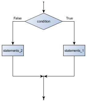
The syntax for an if statement looks like this:
if BOOLEAN EXPRESSION:
    STATEMENTS_1        # Executed if condition evaluates to True
else:
    STATEMENTS_2        # Executed if condition evaluates to False
As with the function definition from the last chapter and other compound statements like for, the if statement consists of a header line and a body. The header line begins with the keyword if followed by a Boolean expression and ends with a colon (:).
The indented statements that follow are called a block. The first unindented statement marks the end of the block.
Each of the statements inside the first block of statements are executed in order if the Boolean expression evaluates to True. The entire first block of statements is skipped if the Boolean expression evaluates to False, and instead all the statements indented under the else clause are executed.
There is no limit on the number of statements that can appear under the two clauses of an if statement, but there has to be at least one statement in each block. Occasionally, it is useful to have a section with no statements (usually as a place keeper, or scaffolding, for code we haven't written yet). In that case, we can use the pass statement, which does nothing except act as a placeholder.
if True:          # This is always True,
    pass          #   so this is always executed, but it does nothing
else:
    pass
Omitting the else clause
Flowchart of an if statement with no else clause
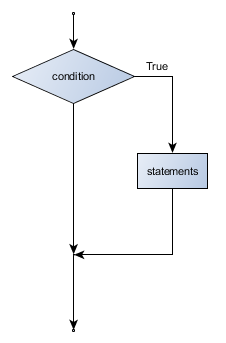
Another form of the if statement is one in which the else clause is omitted entirely. In this case, when the condition evaluates to True, the statements are executed, otherwise the flow of execution continues to the statement after the if.
if x < 0:
    print("The negative number ",  x, " is not valid here.")
    x = 42
    print("I've decided to use the number 42 instead.")

print("The square root of ", x, "is", math.sqrt(x))
In this case, the print function that outputs the square root is the one after the if --- not because we left a blank line, but because of the way the code is indented. Note too that the function call math.sqrt(x) will give an error unless we have an import math statement, usually placed near the top of our script.
Python terminology
Python documentation sometimes uses the term suite of statements to mean what we have called a block here. They mean the same thing, and since most other languages and computer scientists use the word block, we'll stick with that.
Notice too that else is not a statement. The if statement has two clauses, one of which is the (optional) else clause.
Chained conditionals
Sometimes there are more than two possibilities and we need more than two branches. One way to express a computation like that is a chained conditional:
if x < y:
    STATEMENTS_A
elif x > y:
    STATEMENTS_B
else:
    STATEMENTS_C
Flowchart of this chained conditional
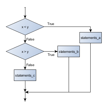
elif is an abbreviation of else if. Again, exactly one branch will be executed. There is no limit of the number of elif statements but only a single (and optional) final else statement is allowed and it must be the last branch in the statement:
if choice == "a":
    function_one()
elif choice == "b":
    function_two()
elif choice == "c":
    function_three()
else:
    print("Invalid choice.")
Each condition is checked in order. If the first is false, the next is checked, and so on. If one of them is true, the corresponding branch executes, and the statement ends. Even if more than one condition is true, only the first true branch executes.
Nested conditionals
One conditional can also be nested within another. (It is the same theme of composability, again!) We could have written the previous example as follows:
Flowchart of this nested conditional
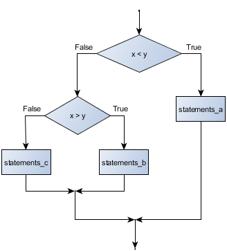
if x < y:
    STATEMENTS_A
else:
    if x > y:
        STATEMENTS_B
    else:
        STATEMENTS_C
The outer conditional contains two branches. The second branch contains another if statement, which has two branches of its own. Those two branches could contain conditional statements as well.
Although the indentation of the statements makes the structure apparent, nested conditionals very quickly become difficult to read. In general, it is a good idea to avoid them when we can.
Logical operators often provide a way to simplify nested conditional statements. For example, we can rewrite the following code using a single conditional:
if 0 < x:            # Assume x is an int here
    if x < 10:
        print("x is a positive single digit.")
The print function is called only if we make it past both the conditionals, so instead of the above which uses two if statements each with a simple condition, we could make a more complex condition using the and operator. Now we only need a single if statement:
if 0 < x and x < 10:
    print("x is a positive single digit.")
The return statement
The return statement, with or without a value, depending on whether the function is fruitful or void, allows us to terminate the execution of a function before (or when) we reach the end. One reason to use an early return is if we detect an error condition:
def print_square_root(x):
    if x <= 0:
        print("Positive numbers only, please.")
        return

    result = x**0.5
    print("The square root of", x, "is", result)
The function print_square_root has a parameter named x. The first thing it does is check whether x is less than or equal to 0, in which case it displays an error message and then uses return to exit the function. The flow of execution immediately returns to the caller, and the remaining lines of the function are not executed.
Logical opposites
Each of the six relational operators has a logical opposite: for example, suppose we can get a driving licence when our age is greater or equal to 17, we can not get the driving licence when we are less than 17.
Notice that the opposite of >= is <.
operator logical opposite == != != == < >= <= > > <= >= <
Understanding these logical opposites allows us to sometimes get rid of not operators. not operators are often quite difficult to read in computer code, and our intentions will usually be clearer if we can eliminate them.
For example, if we wrote this Python:
if not (age >= 17):
    print("Hey, you're too young to get a driving licence!")
it would probably be clearer to use the simplification laws, and to write instead:
if age < 17:
    print("Hey, you're too young to get a driving licence!")
Two powerful simplification laws (called de Morgan's laws) that are often helpful when dealing with complicated Boolean expressions are:
not (x and y)  ==  (not x) or (not y)
not (x or y)   ==  (not x) and (not y)
For example, suppose we can slay the dragon only if our magic lightsabre sword is charged to 90% or higher, and we have 100 or more energy units in our protective shield. We find this fragment of Python code in the game:
if not ((sword_charge >= 0.90) and (shield_energy >= 100)):
    print("Your attack has no effect, the dragon fries you to a crisp!")
else:
    print("The dragon crumples in a heap. You rescue the gorgeous princess!")
de Morgan's laws together with the logical opposites would let us rework the condition in a (perhaps) easier to understand way like this:
if (sword_charge < 0.90) or (shield_energy < 100):
    print("Your attack has no effect, the dragon fries you to a crisp!")
else:
    print("The dragon crumples in a heap. You rescue the gorgeous princess!")
We could also get rid of the not by swapping around the then and else parts of the conditional. So here is a third version, also equivalent:
if (sword_charge >= 0.90) and (shield_energy >= 100):
    print("The dragon crumples in a heap. You rescue the gorgeous princess!")
else:
    print("Your attack has no effect, the dragon fries you to a crisp!")
This version is probably the best of the three, because it very closely matches the initial English statement. Clarity of our code (for other humans), and making it easy to see that the code does what was expected should always be a high priority.
As our programming skills develop we'll find we have more than one way to solve any problem. So good programs are designed. We make choices that favour clarity, simplicity, and elegance. The job title software architect says a lot about what we do --- we are architects who engineer our products to balance beauty, functionality, simplicity and clarity in our creations.
Tip
Once our program works, we should play around a bit trying to polish it up. Write good comments. Think about whether the code would be clearer with different variable names. Could we have done it more elegantly? Should we rather use a function? Can we simplify the conditionals?
We think of our code as our creation, our work of art! We make it great.
Type conversion
We've had a first look at this in an earlier chapter. Seeing it again won't hurt!
Many Python types come with a built-in function that attempts to convert values of another type into its own type. The int function, for example, takes any value and converts it to an integer, if possible, or complains otherwise:
>>> int("32")
32
>>> int("Hello")
ValueError: invalid literal for int() with base 10: 'Hello'
int can also convert floating-point values to integers, but remember that it truncates the fractional part:
>>> int(-2.3)
-2
>>> int(3.99999)
3
>>> int("42")
42
>>> int(1.0)
1
The float function converts integers and strings to floating-point numbers:
>>> float(32)
32.0
>>> float("3.14159")
3.14159
>>> float(1)
1.0
It may seem odd that Python distinguishes the integer value 1 from the floating-point value 1.0. They may represent the same number, but they belong to different types. The reason is that they are represented differently inside the computer.
The str function converts any argument given to it to type string:
>>> str(32)
'32'
>>> str(3.14149)
'3.14149'
>>> str(True)
'True'
>>> str(true)
Traceback (most recent call last):
  File "<interactive input>", line 1, in <module>
NameError: name 'true' is not defined
str will work with any value and convert it into a string. As mentioned earlier, True is Boolean value; true is just an ordinary variable name, and is not defined here, so we get an error.
A Turtle Bar Chart
The turtle has a lot more power than we've seen so far. The full documentation can be found at http://docs.python.org/py3k/library/turtle.html or within PyScripter, use Help and search for the turtle module.
Here are a couple of new tricks for our turtles:
- We can get a turtle to display text on the canvas at the turtle's current position. The method to do that is alex.write("Hello").
- We can fill a shape (circle, semicircle, triangle, etc.) with a color. It is a two-step process. First we call the method alex.begin_fill(), then we draw the shape, then we call alex.end_fill().
- We've previously set the color of our turtle --- we can now also set its fill color, which need not be the same as the turtle and the pen color. We use alex.color("blue","red") to set the turtle to draw in blue, and fill in red.
Ok, so can we get tess to draw a bar chart? Let us start with some data to be charted,
xs = [48, 117, 200, 240, 160, 260, 220]
Corresponding to each data measurement, we'll draw a simple rectangle of that height, with a fixed width.
def draw_bar(t, height):
    """ Get turtle t to draw one bar, of height. """
    t.left(90)
    t.forward(height)     # Draw up the left side
    t.right(90)
    t.forward(40)         # Width of bar, along the top
    t.right(90)
    t.forward(height)     # And down again!
    t.left(90)            # Put the turtle facing the way we found it.
    t.forward(10)         # Leave small gap after each bar

...
for v in xs:              # Assume xs and tess are ready
    draw_bar(tess, v)
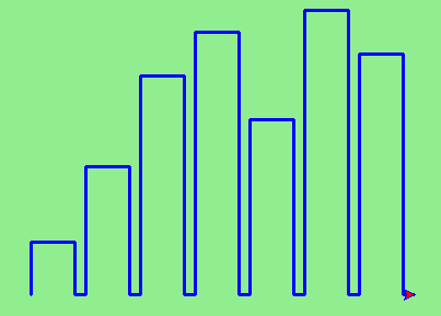
Ok, not fantasically impressive, but it is a nice start! The important thing here was the mental chunking, or how we broke the problem into smaller pieces. Our chunk is to draw one bar, and we wrote a function to do that. Then, for the whole chart, we repeatedly called our function.
Next, at the top of each bar, we'll print the value of the data. We'll do this in the body of draw_bar, by adding t.write(' ' + str(height)) as the new third line of the body. We've put a little space in front of the number, and turned the number into a string. Without this extra space we tend to cramp our text awkwardly against the bar to the left. The result looks a lot better now:
And now we'll add two lines to fill each bar. Our final program now looks like this:
def draw_bar(t, height):
    """ Get turtle t to draw one bar, of height. """
    t.begin_fill()           # Added this line
    t.left(90)
    t.forward(height)
    t.write("  "+ str(height))
    t.right(90)
    t.forward(40)
    t.right(90)
    t.forward(height)
    t.left(90)
    t.end_fill()             # Added this line
    t.forward(10)

wn = turtle.Screen()         # Set up the window and its attributes
wn.bgcolor("lightgreen")

tess = turtle.Turtle()       # Create tess and set some attributes
tess.color("blue", "red")
tess.pensize(3)

xs = [48,117,200,240,160,260,220]

for a in xs:
    draw_bar(tess, a)

wn.mainloop()
It produces the following, which is more satisfying:
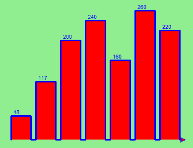
Mmm. Perhaps the bars should not be joined to each other at the bottom. We'll need to pick up the pen while making the gap between the bars. We'll leave that as an exercise for you!
Glossary
- block
- A group of consecutive statements with the same indentation.
- body
- The block of statements in a compound statement that follows the header.
- Boolean algebra
- Some rules for rearranging and reasoning about Boolean expressions.
- Boolean expression
- An expression that is either true or false.
- Boolean value
- There are exactly two Boolean values: True and False. Boolean values result when a Boolean expression is evaluated by the Python interepreter. They have type bool.
- branch
- One of the possible paths of the flow of execution determined by conditional execution.
- chained conditional
- A conditional branch with more than two possible flows of execution. In Python chained conditionals are written with if ... elif ... else statements.
- comparison operator
- One of the six operators that compares two values: ==, !=, >, <, >=, and <=.
- condition
- The Boolean expression in a conditional statement that determines which branch is executed.
- conditional statement
- A statement that controls the flow of execution depending on some condition. In Python the keywords if, elif, and else are used for conditional statements.
- logical operator
- One of the operators that combines Boolean expressions: and, or, and not.
- nesting
- One program structure within another, such as a conditional statement inside a branch of another conditional statement.
- prompt
- A visual cue that tells the user that the system is ready to accept input data.
- truth table
- A concise table of Boolean values that can describe the semantics of an operator.
- type conversion
- An explicit function call that takes a value of one type and computes a corresponding value of another type.
- wrapping code in a function
- The process of adding a function header and parameters to a sequence of program statements is often refered to as "wrapping the code in a function". This process is very useful whenever the program statements in question are going to be used multiple times. It is even more useful when it allows the programmer to express their mental chunking, and how they've broken a complex problem into pieces.
References
| [ThinkCS] | How To Think Like a Computer Scientist --- Learning with Python 3 |
Fruitful functions
Source: this section is heavily based on Chapter 6 of [ThinkCS].
Return values
The built-in functions we have used, such as abs, pow, int, max, and range, have produced results. Calling each of these functions generates a value, which we usually assign to a variable or use as part of an expression.
biggest = max(3, 7, 2, 5)
x = abs(3 - 11) + 10
We also wrote our own function to return the final amount for a compound interest calculation.
In this chapter, we are going to write more functions that return values, which we will call fruitful functions, for want of a better name. The first example is area, which returns the area of a circle with the given radius:
def area(radius):
    b = 3.14159 * radius**2
    return b
We have seen the return statement before, but in a fruitful function the return statement includes a return value. This statement means: evaluate the return expression, and then return it immediately as the result (the fruit) of this function. The expression provided can be arbitrarily complicated, so we could have written this function like this:
def area(radius):
    return 3.14159 * radius * radius
On the other hand, temporary variables like b above often make debugging easier.
Sometimes it is useful to have multiple return statements, one in each branch of a conditional. We have already seen the built-in abs, now we see how to write our own:
def absolute_value(x):
    if x < 0:
        return -x
    else:
        return x
Another way to write the above function is to leave out the else and just follow the if condition by the second return statement.
def absolute_value(x):
    if x < 0:
        return -x
    return x
Think about this version and convince yourself it works the same as the first one.
Code that appears after a return statement, or any other place the flow of execution can never reach, is called dead code, or unreachable code.
In a fruitful function, it is a good idea to ensure that every possible path through the program hits a return statement. The following version of absolute_value fails to do this:
def bad_absolute_value(x):
    if x < 0:
        return -x
    elif x > 0:
        return x
This version is not correct because if x happens to be 0, neither condition is true, and the function ends without hitting a return statement. In this case, the return value is a special value called None:
>>> print(bad_absolute_value(0))
None
All Python functions return None whenever they do not return another value.
It is also possible to use a return statement in the middle of a for loop, in which case control immediately returns from the function. Let us assume that we want a function which looks through a list of words. It should return the first 2-letter word. If there is not one, it should return the empty string:
def find_first_2_letter_word(xs):
    for wd in xs:
        if len(wd) == 2:
           return wd
    return ""
>>> find_first_2_letter_word(["This", "is", "a", "dead", "parrot"]) 'is' >>> find_first_2_letter_word(["I", "like", "cheese"]) ''
Single-step through this code and convince yourself that in the first test case that we've provided, the function returns while processing the second element in the list: it does not have to traverse the whole list.
Program development
At this point, you should be able to look at complete functions and tell what they do. Also, if you have been doing the exercises, you have written some small functions. As you write larger functions, you might start to have more difficulty, especially with runtime and semantic errors.
To deal with increasingly complex programs, we are going to suggest a technique called incremental development. The goal of incremental development is to avoid long debugging sessions by adding and testing only a small amount of code at a time.
As an example, suppose we want to find the distance between two points, given by the coordinates (x1, y1) and (x2, y2). By the Pythagorean theorem, the distance is:
The first step is to consider what a distance function should look like in Python. In other words, what are the inputs (parameters) and what is the output (return value)?
In this case, the two points are the inputs, which we can represent using four parameters. The return value is the distance, which is a floating-point value.
Already we can write an outline of the function that captures our thinking so far:
def distance(x1, y1, x2, y2):
    return 0.0
Obviously, this version of the function doesn't compute distances; it always returns zero. But it is syntactically correct, and it will run, which means that we can test it before we make it more complicated.
To test the new function, we call it with sample values:
>>> distance(1, 2, 4, 6)
0.0
We chose these values so that the horizontal distance equals 3 and the vertical distance equals 4; that way, the result is 5 (the hypotenuse of a 3-4-5 triangle). When testing a function, it is useful to know the right answer.
At this point we have confirmed that the function is syntactically correct, and we can start adding lines of code. After each incremental change, we test the function again. If an error occurs at any point, we know where it must be --- in the last line we added.
A logical first step in the computation is to find the differences x2- x1 and y2- y1. We will refer to those values using temporary variables named dx and dy.
def distance(x1, y1, x2, y2):
    dx = x2 - x1
    dy = y2 - y1
    return 0.0
If we call the function with the arguments shown above, when the flow of execution gets to the return statement, dx should be 3 and dy should be 4. We can check that this is the case in PyScripter by putting the cursor on the return statement, and running the program to break execution when it gets to the cursor (using the F4 key). Then we inspect the variables dx and dy by hovering the mouse above them, to confirm that the function is getting the right parameters and performing the first computation correctly. If not, there are only a few lines to check.
Next we compute the sum of squares of dx and dy:
def distance(x1, y1, x2, y2):
    dx = x2 - x1
    dy = y2 - y1
    dsquared = dx*dx + dy*dy
    return 0.0
Again, we could run the program at this stage and check the value of dsquared (which should be 25).
Finally, using the fractional exponent 0.5 to find the square root, we compute and return the result:
def distance(x1, y1, x2, y2):
    dx = x2 - x1
    dy = y2 - y1
    dsquared = dx*dx + dy*dy
    result = dsquared**0.5
    return result
If that works correctly, you are done. Otherwise, you might want to inspect the value of result before the return statement.
When you start out, you might add only a line or two of code at a time. As you gain more experience, you might find yourself writing and debugging bigger conceptual chunks. Either way, stepping through your code one line at a time and verifying that each step matches your expectations can save you a lot of debugging time. As you improve your programming skills you should find yourself managing bigger and bigger chunks: this is very similar to the way we learned to read letters, syllables, words, phrases, sentences, paragraphs, etc., or the way we learn to chunk music --- from individual notes to chords, bars, phrases, and so on.
The key aspects of the process are:
- Start with a working skeleton program and make small incremental changes. At any point, if there is an error, you will know exactly where it is.
- Use temporary variables to refer to intermediate values so that you can easily inspect and check them.
- Once the program is working, relax, sit back, and play around with your options. (There is interesting research that links "playfulness" to better understanding, better learning, more enjoyment, and a more positive mindset about what you can achieve --- so spend some time fiddling around!) You might want to consolidate multiple statements into one bigger compound expression, or rename the variables you've used, or see if you can make the function shorter. A good guideline is to aim for making code as easy as possible for others to read.
Here is another version of the function. It makes use of a square root function that is in the math module (we'll learn about modules shortly). Which do you prefer? Which looks "closer" to the Pythagorean formula we started out with?
import math

def distance(x1, y1, x2, y2):
    return math.sqrt( (x2-x1)**2 + (y2-y1)**2 )
>>> distance(1, 2, 4, 6) 5.0
Debugging with print
Another powerful technique for debugging (an alternative to single-stepping and inspection of program variables), is to insert extra print functions in carefully selected places in your code. Then, by inspecting the output of the program, you can check whether the algorithm is doing what you expect it to. Be clear about the following, however:
You must have a clear solution to the problem, and must know what should happen before you can debug a program. Work on solving the problem on a piece of paper (perhaps using a flowchart to record the steps you take) before you concern yourself with writing code. Writing a program doesn't solve the problem --- it simply automates the manual steps you would take. So first make sure you have a pen-and-paper manual solution that works. Programming then is about making those manual steps happen automatically.
Do not write chatterbox functions. A chatterbox is a fruitful function that, in addition to its primary task, also asks the user for input, or prints output, when it would be more useful if it simply shut up and did its work quietly.
For example, we've seen built-in functions like range, max and abs. None of these would be useful building blocks for other programs if they prompted the user for input, or printed their results while they performed their tasks.
So a good tip is to avoid calling print and input functions inside fruitful functions, unless the primary purpose of your function is to perform input and output. The one exception to this rule might be to temporarily sprinkle some calls to print into your code to help debug and understand what is happening when the code runs, but these will then be removed once you get things working.
Composition
As you should expect by now, you can call one function from within another. This ability is called composition.
As an example, we'll write a function that takes two points, the center of the circle and a point on the perimeter, and computes the area of the circle.
Assume that the center point is stored in the variables xc and yc, and the perimeter point is in xp and yp. The first step is to find the radius of the circle, which is the distance between the two points. Fortunately, we've just written a function, distance, that does just that, so now all we have to do is use it:
radius = distance(xc, yc, xp, yp)
The second step is to find the area of a circle with that radius and return it. Again we will use one of our earlier functions:
result = area(radius)
return result
Wrapping that up in a function, we get:
def area2(xc, yc, xp, yp):
    radius = distance(xc, yc, xp, yp)
    result = area(radius)
    return result
We called this function area2 to distinguish it from the area function defined earlier.
The temporary variables radius and result are useful for development, debugging, and single-stepping through the code to inspect what is happening, but once the program is working, we can make it more concise by composing the function calls:
def area2(xc, yc, xp, yp):
    return area(distance(xc, yc, xp, yp))
Boolean functions
Functions can return Boolean values, which is often convenient for hiding complicated tests inside functions. For example:
def is_divisible(x, y):
    """ Test if x is exactly divisible by y """
    if x % y == 0:
        return True
    else:
        return False
It is common to give Boolean functions names that sound like yes/no questions. is_divisible returns either True or False to indicate whether the x is or is not divisible by y.
We can make the function more concise by taking advantage of the fact that the condition of the if statement is itself a Boolean expression. We can return it directly, avoiding the if statement altogether:
def is_divisible(x, y):
    return x % y == 0
This session shows the new function in action:
>>> is_divisible(6, 4)
False
>>> is_divisible(6, 3)
True
Boolean functions are often used in conditional statements:
if is_divisible(x, y):
    ... # Do something ...
else:
    ... # Do something else ...
It might be tempting to write something like:
if is_divisible(x, y) == True:
but the extra comparison is unnecessary.
Programming with style
Readability is very important to programmers, since in practice programs are read and modified far more often then they are written. But, like most rules, we occasionaly break them. Most of the code examples in this book will be consistent with the Python Enhancement Proposal 8 (PEP 8), a style guide developed by the Python community.
We'll have more to say about style as our programs become more complex, but a few pointers will be helpful already:
- use 4 spaces (instead of tabs) for indentation
- limit line length to 78 characters
- when naming identifiers, use CamelCase for classes (we'll get to those) and lowercase_with_underscores for functons and variables
- place imports at the top of the file
- keep function definitions together
- use docstrings to document functions
- use two blank lines to separate function definitions from each other
- keep top level statements, including function calls, together at the bottom of the program
Unit testing
It is a common best practice in software development to include automatic unit testing of source code. Unit testing provides a way to automatically verify that individual pieces of code, such as functions, are working properly. This makes it possible to change the implementation of a function at a later time and quickly test that it still does what it was intended to do.
Some years back organizations had the view that their valuable asset was the program code and documentation. Organizations will now spend a large portion of their software budgets on crafting (and preserving) their tests.
Unit testing also forces the programmer to think about the different cases that the function needs to handle. You also only have to type the tests once into the script, rather than having to keep entering the same test data over and over as you develop your code.
Extra code in your program which is there because it makes debugging or testing easier is called scaffolding.
A collection of tests for some code is called its test suite.
There are a few different ways to do unit testing in Python --- but at this stage we're going to ignore what the Python community usually does, and we're going to start with two functions that we'll write ourselves. We'll use these for writing our unit tests.
Let's start with the absolute_value function that we wrote earlier in this chapter. Recall that we wrote a few different versions, the last of which was incorrect, and had a bug. Would tests have caught this bug?
First we plan our tests. We'd like to know if the function returns the correct value when its argument is negative, or when its argument is positive, or when its argument is zero. When planning your tests, you'll always want to think carefully about the "edge" cases --- here, an argument of 0 to absolute_value is on the edge of where the function behaviour changes, and as we saw at the beginning of the chapter, it is an easy spot for the programmer to make a mistake! So it is a good case to include in our test suite.
We're going to write a helper function for checking the results of one test. It takes a boolean argument and will either print a message telling us that the test passed, or it will print a message to inform us that the test failed. The first line of the body (after the function's docstring) magically determines the line number in the script where the call was made from. This allows us to print the line number of the test, which will help when we want to identify which tests have passed or failed.
import sys

def test(did_pass):
    """  Print the result of a test.  """
    linenum = sys._getframe(1).f_lineno   # Get the caller's line number.
    if did_pass:
        msg = "Test at line {0} ok.".format(linenum)
    else:
        msg = ("Test at line {0} FAILED.".format(linenum))
    print(msg)
There is also some slightly tricky string formatting using the format method which we will gloss over for the moment, and cover in detail in a future chapter. But with this function written, we can proceed to construct our test suite:
def test_suite():
    """ Run the suite of tests for code in this module (this file).
    """
    test(absolute_value(17) == 17)
    test(absolute_value(-17) == 17)
    test(absolute_value(0) == 0)
    test(absolute_value(3.14) == 3.14)
    test(absolute_value(-3.14) == 3.14)

test_suite()        # Here is the call to run the tests
Here you'll see that we've constructed five tests in our test suite. We could run this against the first or second versions (the correct versions) of absolute_value, and we'd get output similar to the following:
Test at line 25 ok.
Test at line 26 ok.
Test at line 27 ok.
Test at line 28 ok.
Test at line 29 ok.
But let's say you change the function to an incorrect version like this:
def absolute_value(n):   # Buggy version
    """ Compute the absolute value of n """
    if n < 0:
        return 1
    elif n > 0:
        return n
Can you find at least two mistakes in this code? Our test suite can! We get:
Test at line 25 ok.
Test at line 26 FAILED.
Test at line 27 FAILED.
Test at line 28 ok.
Test at line 29 FAILED.
These are three examples of failing tests.
There is a built-in Python statement called assert that does almost the same as our test function (except the program stops when the first assertion fails). You may want to read about it, and use it instead of our test function.
Glossary
- Boolean function
- A function that returns a Boolean value. The only possible values of the bool type are False and True.
- chatterbox function
- A function which interacts with the user (using input or print) when it should not. Silent functions that just convert their input arguments into their output results are usually the most useful ones.
- composition (of functions)
- Calling one function from within the body of another, or using the return value of one function as an argument to the call of another.
- dead code
- Part of a program that can never be executed, often because it appears after a return statement.
- fruitful function
- A function that yields a return value instead of None.
- incremental development
- A program development plan intended to simplify debugging by adding and testing only a small amount of code at a time.
- None
- A special Python value. One use in Python is that it is returned by functions that do not execute a return statement with a return argument.
- return value
- The value provided as the result of a function call.
- scaffolding
- Code that is used during program development to assist with development and debugging. The unit test code that we added in this chapter are examples of scaffolding.
- temporary variable
- A variable used to store an intermediate value in a complex calculation.
- test suite
- A collection of tests for some code you have written.
- unit testing
- An automatic procedure used to validate that individual units of code are working properly. Having a test suite is extremely useful when somebody modifies or extends the code: it provides a safety net against going backwards by putting new bugs into previously working code. The term regression testing is often used to capture this idea that we don't want to go backwards!
References
| [ThinkCS] | How To Think Like a Computer Scientist --- Learning with Python 3 |
Iteration
Source: this section is heavily based on Chapter 7 of [ThinkCS].
Computers are often used to automate repetitive tasks. Repeating identical or similar tasks without making errors is something that computers do well and people do poorly.
Repeated execution of a set of statements is called iteration. Because iteration is so common, Python provides several language features to make it easier. We've already seen the for statement in chapter 3. This the the form of iteration you'll likely be using most often. But in this chapter we've going to look at the while statement --- another way to have your program do iteration, useful in slightly different circumstances.
Before we do that, let's just review a few ideas...
Assignment
As we have mentioned previously, it is legal to make more than one assignment to the same variable. A new assignment makes an existing variable refer to a new value (and stop referring to the old value).
airtime_remaining = 15
print(airtime_remaining)
airtime_remaining = 7
print(airtime_remaining)
The output of this program is:
15
7
because the first time airtime_remaining is printed, its value is 15, and the second time, its value is 7.
It is especially important to distinguish between an assignment statement and a Boolean expression that tests for equality. Because Python uses the equal token (=) for assignment, it is tempting to interpret a statement like a = b as a Boolean test. Unlike mathematics, it is not! Remember that the Python token for the equality operator is ==.
Note too that an equality test is symmetric, but assignment is not. For example, if a == 7 then 7 == a. But in Python, the statement a = 7 is legal and 7 = a is not.
In Python, an assignment statement can make two variables equal, but because further assignments can change either of them, they don't have to stay that way:
a = 5
b = a    # After executing this line, a and b are now equal
a = 3    # After executing this line, a and b are no longer equal
The third line changes the value of a but does not change the value of b, so they are no longer equal. (In some programming languages, a different symbol is used for assignment, such as <- or :=, to avoid confusion. Some people also think that variable was an unfortunae word to choose, and instead we should have called them assignables. Python chooses to follow common terminology and token usage, also found in languages like C, C++, Java, and C#, so we use the tokens = for assignment, == for equality, and we talk of variables.
Updating variables
When an assignment statement is executed, the right-hand side expression (i.e. the expression that comes after the assignment token) is evaluated first. This produces a value. Then the assignment is made, so that the variable on the left-hand side now refers to the new value.
One of the most common forms of assignment is an update, where the new value of the variable depends on its old value. Deduct 40 cents from my airtime balance, or add one run to the scoreboard.
n = 5
n = 3 * n + 1
Line 2 means get the current value of n, multiply it by three and add one, and assign the answer to n, thus making n refer to the value. So after executing the two lines above, n will point/refer to the integer 16.
If you try to get the value of a variable that has never been assigned to, you'll get an error:
>>> w = x + 1
Traceback (most recent call last):
  File "<interactive input>", line 1, in
NameError: name 'x' is not defined
Before you can update a variable, you have to initialize it to some starting value, usually with a simple assignment:
runs_scored = 0
...
runs_scored = runs_scored + 1
Line 3 --- updating a variable by adding 1 to it --- is very common. It is called an increment of the variable; subtracting 1 is called a decrement. Sometimes programmers also talk about bumping a variable, which means the same as incrementing it by 1.
The for loop revisited
Recall that the for loop processes each item in a list. Each item in turn is (re-)assigned to the loop variable, and the body of the loop is executed. We saw this example in an earlier chapter:
for f in ["Joe", "Zoe", "Brad", "Angelina", "Zuki", "Thandi", "Paris"]:
    invitation = "Hi " + f + ".  Please come to my party on Saturday!"
    print(invitation)
Running through all the items in a list is called traversing the list, or traversal.
Let us write a function now to sum up all the elements in a list of numbers. Do this by hand first, and try to isolate exactly what steps you take. You'll find you need to keep some "running total" of the sum so far, either on a piece of paper, in your head, or in your calculator. Remembering things from one step to the next is precisely why we have variables in a program: so we'll need some variable to remember the "running total". It should be initialized with a value of zero, and then we need to traverse the items in the list. For each item, we'll want to update the running total by adding the next number to it.
def mysum(xs):
    """ Sum all the numbers in the list xs, and return the total. """
    running_total = 0
    for x in xs:
        running_total = running_total + x
    return running_total

# Add tests like these to your test suite ...
test(mysum([1, 2, 3, 4]) == 10)
test(mysum([1.25, 2.5, 1.75]) == 5.5)
test(mysum([1, -2, 3]) == 2)
test(mysum([ ]) == 0)
test(mysum(range(11)) == 55)  # 11 is not included in the list.
The while statement
Here is a fragment of code that demonstrates the use of the while statement:
def sum_to(n):
    """ Return the sum of 1+2+3 ... n """
    ss  = 0
    v = 1
    while v <= n:
        ss = ss + v
        v = v + 1
    return ss

# For your test suite
test(sum_to(4) == 10)
test(sum_to(1000) == 500500)
You can almost read the while statement as if it were English. It means, while v is less than or equal to n, continue executing the body of the loop. Within the body, each time, increment v. When v passes n, return your accumulated sum.
More formally, here is precise flow of execution for a while statement:
- Evaluate the condition at line 5, yielding a value which is either False or True.
- If the value is False, exit the while statement and continue execution at the next statement (line 8 in this case).
- If the value is True, execute each of the statements in the body (lines 6 and 7) and then go back to the while statement at line 5.
The body consists of all of the statements indented below the while keyword.
Notice that if the loop condition is False the first time we get loop, the statements in the body of the loop are never executed.
The body of the loop should change the value of one or more variables so that eventually the condition becomes false and the loop terminates. Otherwise the loop will repeat forever, which is called an infinite loop. An endless source of amusement for computer scientists is the observation that the directions on shampoo, "lather, rinse, repeat", are an infinite loop.
In the case here, we can prove that the loop terminates because we know that the value of n is finite, and we can see that the value of v increments each time through the loop, so eventually it will have to exceed n. In other cases, it is not so easy, even impossible in some cases, to tell if the loop will ever terminate.
What you will notice here is that the while loop is more work for you --- the programmer --- than the equivalent for loop. When using a while loop one has to manage the loop variable yourself: give it an initial value, test for completion, and then make sure you change something in the body so that the loop terminates. By comparison, here is an equivalent function that uses for instead:
def sum_to(n):
    """ Return the sum of 1+2+3 ... n """
    ss  = 0
    for v in range(n+1):
        ss = ss + v
    return ss
Notice the slightly tricky call to the range function --- we had to add one onto n, because range generates its list up to but excluding the value you give it. It would be easy to make a programming mistake and overlook this, but because we've made the investment of writing some unit tests, our test suite would have caught our error.
So why have two kinds of loop if for looks easier? This next example shows a case where we need the extra power that we get from the while loop.
The Collatz 3n + 1 sequence
Let's look at a simple sequence that has fascinated and foxed mathematicians for many years. They still cannot answer even quite simple questions about this.
The "computational rule" for creating the sequence is to start from some given n, and to generate the next term of the sequence from n, either by halving n, (whenever n is even), or else by multiplying it by three and adding 1. The sequence terminates when n reaches 1.
This Python function captures that algorithm:
def seq3np1(n):
    """ Print the 3n+1 sequence from n,
        terminating when it reaches 1.
    """
    while n != 1:
        print(n, end=", ")
        if n % 2 == 0:        # n is even
            n = n // 2
        else:                 # n is odd
            n = n * 3 + 1
    print(n, end=".\n")
Notice first that the print function on line 6 has an extra argument end=", ". This tells the print function to follow the printed string with whatever the programmer chooses (in this case, a comma followed by a space), instead of ending the line. So each time something is printed in the loop, it is printed on the same output line, with the numbers separated by commas. The call to print(n, end=".\n") at line 11 after the loop terminates will then print the final value of n followed by a period and a newline character. (You'll cover the \n (newline character) in the next chapter).
The condition for continuing with this loop is n != 1, so the loop will continue running until it reaches its termination condition, (i.e. n == 1).
Each time through the loop, the program outputs the value of n and then checks whether it is even or odd. If it is even, the value of n is divided by 2 using integer division. If it is odd, the value is replaced by n * 3 + 1. Here are some examples:
>>> seq3np1(3)
3, 10, 5, 16, 8, 4, 2, 1.
>>> seq3np1(19)
19, 58, 29, 88, 44, 22, 11, 34, 17, 52, 26, 13,
                    40, 20, 10, 5, 16, 8, 4, 2, 1.
>>> seq3np1(21)
21, 64, 32, 16, 8, 4, 2, 1.
>>> seq3np1(16)
16, 8, 4, 2, 1.
>>>
Since n sometimes increases and sometimes decreases, there is no obvious proof that n will ever reach 1, or that the program terminates. For some particular values of n, we can prove termination. For example, if the starting value is a power of two, then the value of n will be even each time through the loop until it reaches 1. The previous example ends with such a sequence, starting with 16.
See if you can find a small starting number that needs more than a hundred steps before it terminates.
Particular values aside, the interesting question was first posed by a German mathematician called Lothar Collatz: the Collatz conjecture (also known as the 3n + 1 conjecture), is that this sequence terminates for all positive values of n. So far, no one has been able to prove it or disprove it! (A conjecture is a statement that might be true, but nobody knows for sure.)
Think carefully about what would be needed for a proof or disproof of the conjecture "All positive integers will eventually converge to 1 using the Collatz rules". With fast computers we have been able to test every integer up to very large values, and so far, they have all eventually ended up at 1. But who knows? Perhaps there is some as-yet untested number which does not reduce to 1.
You'll notice that if you don't stop when you reach 1, the sequence gets into its own cyclic loop: 1, 4, 2, 1, 4, 2, 1, 4 ... So one possibility is that there might be other cycles that we just haven't found yet.
Wikipedia has an informative article about the Collatz conjecture. The sequence also goes under other names (Hailstone sequence, Wonderous numbers, etc.), and you'll find out just how many integers have already been tested by computer, and found to converge!
Choosing between for and while
Use a for loop if you know, before you start looping, the maximum number of times that you'll need to execute the body. For example, if you're traversing a list of elements, you know that the maximum number of loop iterations you can possibly need is "all the elements in the list". Or if you need to print the 12 times table, we know right away how many times the loop will need to run.
So any problem like "iterate this weather model for 1000 cycles", or "search this list of words", "find all prime numbers up to 10000" suggest that a for loop is best.
By contrast, if you are required to repeat some computation until some condition is met, and you cannot calculate in advance when (of if) this will happen, as we did in this 3n + 1 problem, you'll need a while loop.
We call the first case definite iteration --- we know ahead of time some definite bounds for what is needed. The latter case is called indefinite iteration --- we're not sure how many iterations we'll need --- we cannot even establish an upper bound!
Tracing a program
To write effective computer programs, and to build a good conceptual model of program execution, a programmer needs to develop the ability to trace the execution of a computer program. Tracing involves becoming the computer and following the flow of execution through a sample program run, recording the state of all variables and any output the program generates after each instruction is executed.
To understand this process, let's trace the call to seq3np1(3) from the previous section. At the start of the trace, we have a variable, n (the parameter), with an initial value of 3. Since 3 is not equal to 1, the while loop body is executed. 3 is printed and 3 % 2 == 0 is evaluated. Since it evaluates to False, the else branch is executed and 3 * 3 + 1 is evaluated and assigned to n.
To keep track of all this as you hand trace a program, make a column heading on a piece of paper for each variable created as the program runs and another one for output. Our trace so far would look something like this:
n               output printed so far
--              ---------------------
3               3,
10
Since 10 != 1 evaluates to True, the loop body is again executed, and 10 is printed. 10 % 2 == 0 is true, so the if branch is executed and n becomes 5. By the end of the trace we have:
n               output printed so far
--              ---------------------
3               3,
10              3, 10,
5               3, 10, 5,
16              3, 10, 5, 16,
8               3, 10, 5, 16, 8,
4               3, 10, 5, 16, 8, 4,
2               3, 10, 5, 16, 8, 4, 2,
1               3, 10, 5, 16, 8, 4, 2, 1.
Tracing can be a bit tedious and error prone (that's why we get computers to do this stuff in the first place!), but it is an essential skill for a programmer to have. From this trace we can learn a lot about the way our code works. We can observe that as soon as n becomes a power of 2, for example, the program will require log2(n) executions of the loop body to complete. We can also see that the final 1 will not be printed as output within the body of the loop, which is why we put the special print function at the end.
Tracing a program is, of course, related to single-stepping through your code and being able to inspect the variables. Using the computer to single-step for you is less error prone and more convenient. Also, as your programs get more complex, they might execute many millions of steps before they get to the code that you're really interested in, so manual tracing becomes impossible. Being able to set a breakpoint where you need one is far more powerful. So we strongly encourage you to invest time in learning using to use your programming environment (PyScripter, in these notes) to full effect.
There are also some great visualization tools becoming available to help you trace and understand small fragments of Python code. The one we recommend is at http://www.pythontutor.com/visualize.html .
We've cautioned against chatterbox functions, but used them here. As we learn a bit more Python, we'll be able to show you how to generate a list of values to hold the sequence, rather than having the function print them. Doing this would remove the need to have all these pesky print functions in the middle of our logic, and will make the function more useful.
Counting digits
The following function counts the number of decimal digits in a positive integer:
def num_digits(n):
    count = 0
    while n != 0:
        count = count + 1
        n = n // 10
    return count
A call to print(num_digits(710)) will print 3. Trace the execution of this function call (perhaps using the single step function in PyScripter, or the Python visualizer, or on some paper) to convince yourself that it works.
This function demonstrates an important pattern of computation called a counter. The variable count is initialized to 0 and then incremented each time the loop body is executed. When the loop exits, count contains the result --- the total number of times the loop body was executed, which is the same as the number of digits.
If we wanted to only count digits that are either 0 or 5, adding a conditional before incrementing the counter will do the trick:
def num_zero_and_five_digits(n):
    count = 0
    while n > 0:
        digit = n % 10
        if digit == 0 or digit == 5:
            count = count + 1
        n = n // 10
    return count
Confirm that test(num_zero_and_five_digits(1055030250) == 7) passes.
Notice, however, that test(num_digits(0) == 1) fails. Explain why. Do you think this is a bug in the code, or a bug in the specifications, or our expectations, or the tests?
Abbreviated assignment
Incrementing a variable is so common that Python provides an abbreviated syntax for it:
>>> count = 0
>>> count += 1
>>> count
1
>>> count += 1
>>> count
2
count += 1 is an abreviation for count = count + 1 . We pronounce the operator as "plus-equals". The increment value does not have to be 1:
>>> n = 2
>>> n += 5
>>> n
7
There are similar abbreviations for -=, *=, /=, //= and %=:
>>> n = 2
>>> n *= 5
>>> n
10
>>> n -= 4
>>> n
6
>>> n //= 2
>>> n
3
>>> n %= 2
>>> n
1
Help and meta-notation
Python comes with extensive documentation for all its built-in functions, and its libraries. Different systems have different ways of accessing this help. In PyScripter, click on the Help menu item, and select Python Manuals. Then search for help on the built-in function range. You'll get something like this:
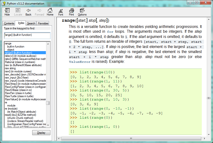
Notice the square brackets in the description of the arguments. These are examples of meta-notation --- notation that describes Python syntax, but is not part of it. The square brackets in this documentation mean that the argument is optional --- the programmer can omit it. So what this first line of help tells us is that range must always have a stop argument, but it may have an optional start argument (which must be followed by a comma if it is present), and it can also have an optional step argument, preceded by a comma if it is present.
The examples from help show that range can have either 1, 2 or 3 arguments. The list can start at any starting value, and go up or down in increments other than 1. The documentation here also says that the arguments must be integers.
Other meta-notation you'll frequently encounter is the use of bold and italics. The bold means that these are tokens --- keywords or symbols --- typed into your Python code exactly as they are, whereas the italic terms stand for "something of this type". So the syntax description
for variable in list :
means you can substitute any legal variable and any legal list when you write your Python code.
This (simplified) description of the print function, shows another example of meta-notation in which the ellipses (...) mean that you can have as many objects as you like (even zero), separated by commas:
print( [object, ... ] )
Meta-notation gives us a concise and powerful way to describe the pattern of some syntax or feature.
Tables
One of the things loops are good for is generating tables. Before computers were readily available, people had to calculate logarithms, sines and cosines, and other mathematical functions by hand. To make that easier, mathematics books contained long tables listing the values of these functions. Creating the tables was slow and boring, and they tended to be full of errors.
When computers appeared on the scene, one of the initial reactions was, "This is great! We can use the computers to generate the tables, so there will be no errors." That turned out to be true (mostly) but shortsighted. Soon thereafter, computers and calculators were so pervasive that the tables became obsolete.
Well, almost. For some operations, computers use tables of values to get an approximate answer and then perform computations to improve the approximation. In some cases, there have been errors in the underlying tables, most famously in the table the Intel Pentium processor chip used to perform floating-point division.
Although a log table is not as useful as it once was, it still makes a good example of iteration. The following program outputs a sequence of values in the left column and 2 raised to the power of that value in the right column:
for x in range(13):   # Generate numbers 0 to 12
    print(x, "\t", 2**x)
The string "\t" represents a tab character. The backslash character in "\t" indicates the beginning of an escape sequence. Escape sequences are used to represent invisible characters like tabs and newlines. The sequence \n represents a newline.
An escape sequence can appear anywhere in a string; in this example, the tab escape sequence is the only thing in the string. How do you think you represent a backslash in a string?
As characters and strings are displayed on the screen, an invisible marker called the cursor keeps track of where the next character will go. After a print function, the cursor normally goes to the beginning of the next line.
The tab character shifts the cursor to the right until it reaches one of the tab stops. Tabs are useful for making columns of text line up, as in the output of the previous program:
0       1
1       2
2       4
3       8
4       16
5       32
6       64
7       128
8       256
9       512
10      1024
11      2048
12      4096
Because of the tab characters between the columns, the position of the second column does not depend on the number of digits in the first column.
Two-dimensional tables
A two-dimensional table is a table where you read the value at the intersection of a row and a column. A multiplication table is a good example. Let's say you want to print a multiplication table for the values from 1 to 6.
A good way to start is to write a loop that prints the multiples of 2, all on one line:
for i in range(1, 7):
    print(2 * i, end="   ")
print()
Here we've used the range function, but made it start its sequence at 1. As the loop executes, the value of i changes from 1 to 6. When all the elements of the range have been assigned to i, the loop terminates. Each time through the loop, it displays the value of 2 * i, followed by three spaces.
Again, the extra end=" " argument in the print function suppresses the newline, and uses three spaces instead. After the loop completes, the call to print at line 3 finishes the current line, and starts a new line.
The output of the program is:
2 4 6 8 10 12
So far, so good. The next step is to encapsulate and generalize.
Encapsulation and generalization
Encapsulation is the process of wrapping a piece of code in a function, allowing you to take advantage of all the things functions are good for. You have already seen some examples of encapsulation, including is_divisible in a previous chapter.
Generalization means taking something specific, such as printing the multiples of 2, and making it more general, such as printing the multiples of any integer.
This function encapsulates the previous loop and generalizes it to print multiples of n:
def print_multiples(n):
    for i in range(1, 7):
        print(n * i, end="   ")
    print()
To encapsulate, all we had to do was add the first line, which declares the name of the function and the parameter list. To generalize, all we had to do was replace the value 2 with the parameter n.
If we call this function with the argument 2, we get the same output as before. With the argument 3, the output is:
3 6 9 12 15 18
With the argument 4, the output is:
4 8 12 16 20 24
By now you can probably guess how to print a multiplication table --- by calling print_multiples repeatedly with different arguments. In fact, we can use another loop:
for i in range(1, 7):
    print_multiples(i)
Notice how similar this loop is to the one inside print_multiples. All we did was replace the print function with a function call.
The output of this program is a multiplication table:
1      2      3      4      5      6
2      4      6      8      10     12
3      6      9      12     15     18
4      8      12     16     20     24
5      10     15     20     25     30
6      12     18     24     30     36
More encapsulation
To demonstrate encapsulation again, let's take the code from the last section and wrap it up in a function:
def print_mult_table():
    for i in range(1, 7):
        print_multiples(i)
This process is a common development plan. We develop code by writing lines of code outside any function, or typing them in to the interpreter. When we get the code working, we extract it and wrap it up in a function.
This development plan is particularly useful if you don't know how to divide the program into functions when you start writing. This approach lets you design as you go along.
Local variables
You might be wondering how we can use the same variable, i, in both print_multiples and print_mult_table. Doesn't it cause problems when one of the functions changes the value of the variable?
The answer is no, because the i in print_multiples and the i in print_mult_table are not the same variable.
Variables created inside a function definition are local; you can't access a local variable from outside its home function. That means you are free to have multiple variables with the same name as long as they are not in the same function.
Python examines all the statements in a function --- if any of them assign a value to a variable, that is the clue that Python uses to make the variable a local variable.
The stack diagram for this program shows that the two variables named i are not the same variable. They can refer to different values, and changing one does not affect the other.
The value of i in print_mult_table goes from 1 to 6. In the diagram it happens to be 3. The next time through the loop it will be 4. Each time through the loop, print_mult_table calls print_multiples with the current value of i as an argument. That value gets assigned to the parameter n.
Inside print_multiples, the value of i goes from 1 to 6. In the diagram, it happens to be 2. Changing this variable has no effect on the value of i in print_mult_table.
It is common and perfectly legal to have different local variables with the same name. In particular, names like i and j are used frequently as loop variables. If you avoid using them in one function just because you used them somewhere else, you will probably make the program harder to read.
The visualizer at http://www.pythontutor.com/visualize.html shows very clearly how the two variables i are distinct variables, and how they have independent values.
The break statement
The break statement is used to immediately leave the body of its loop. The next statement to be executed is the first one after the body:
for i in [12, 16, 17, 24, 29]:
    if i % 2 == 1:  # If the number is odd
       break        #  ... immediately exit the loop
    print(i)
print("done")
This prints:
12
16
done
The pre-test loop --- standard loop behaviour
for and while loops do their tests at the start, before executing any part of the body. They're called pre-test loops, because the test happens before (pre) the body. break and return are our tools for adapting this standard behaviour.
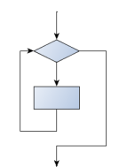
Other flavours of loops
Sometimes we'd like to have the middle-test loop with the exit test in the middle of the body, rather than at the beginning or at the end. Or a post-test loop that puts its exit test as the last thing in the body. Other languages have different syntax and keywords for these different flavours, but Python just uses a combination of while and if condition: break to get the job done.
A typical example is a problem where the user has to input numbers to be summed. To indicate that there are no more inputs, the user enters a special value, often the value -1, or the empty string. This needs a middle-exit loop pattern: input the next number, then test whether to exit, or else process the number:
The middle-test loop flowchart
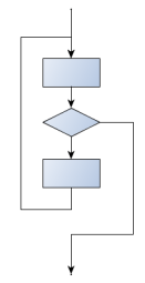
total = 0
while True:
    response = input("Enter the next number. (Leave blank to end)")
    if response == "":
        break
    total += int(response)
print("The total of the numbers you entered is ", total)
Convince yourself that this fits the middle-exit loop flowchart: line 3 does some useful work, lines 4 and 5 can exit the loop, and if they don't line 6 does more useful work before the next iteration starts.
The while bool-expr: uses the Boolean expression to determine whether to iterate again. True is a trivial Boolean expression, so while True: means always do the loop body again. This is a language idiom --- a convention that most programmers will recognize immediately. Since the expression on line 2 will never terminate the loop, (it is a dummy test) the programmer must arrange to break (or return) out of the loop body elsewhere, in some other way (i.e. in lines 4 and 5 in this sample). A clever compiler or interpreter will understand that line 2 is a fake test that must always succeed, so it won't even generate a test, and our flowchart never even put the diamond-shape dummy test box at the top of the loop!
Similarly, by just moving the if condition: break to the end of the loop body we create a pattern for a post-test loop. Post-test loops are used when you want to be sure that the loop body always executes at least once (because the first test only happens at the end of the execution of the first loop body). This is useful, for example, if we want to play an interactive game against the user --- we always want to play at least one game:
while True:
    play_the_game_once()
    response = input("Play again? (yes or no)")
    if response != "yes":
        break
print("Goodbye!")
Hint: Think about where you want the exit test to happen
Once you've recognized that you need a loop to repeat something, think about its terminating condition --- when will I want to stop iterating? Then figure out whether you need to do the test before starting the first (and every other) iteration, or at the end of the first (and every other) iteration, or perhaps in the middle of each iteration. Interactive programs that require input from the user or read from files often need to exit their loops in the middle or at the end of an iteration, when it becomes clear that there is no more data to process, or the user doesn't want to play our game anymore.
An example
The following program implements a simple guessing game:
import random                   # We cover random numbers in the
rng = random.Random()           #  modules chapter, so peek ahead.
number = rng.randrange(1, 1000) # Get random number between [1 and 1000).

guesses = 0
msg = ""

while True:
    guess = int(input(msg + "\nGuess my number between 1 and 1000: "))
    guesses += 1
    if guess > number:
        msg += str(guess) + " is too high.\n"
    elif guess < number:
        msg += str(guess) + " is too low.\n"
    else:
        break

input("\n\nGreat, you got it in {0} guesses!\n\n".format(guesses))
This program makes use of the mathematical law of trichotomy (given real numbers a and b, exactly one of these three must be true: a > b, a < b, or a == b).
At line 18 there is a call to the input function, but we don't do anything with the result, not even assign it to a variable. This is legal in Python. Here it has the effect of popping up the input dialog window and waiting for the user to respond before the program terminates. Programmers often use the trick of doing some extra input at the end of a script, just to keep the window open.
Also notice the use of the msg variable, initially an empty string, on lines 6, 12 and 14. Each time through the loop we extend the message being displayed: this allows us to display the program's feedback right at the same place as we're asking for the next guess.
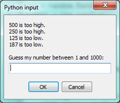
The continue statement
This is a control flow statement that causes the program to immediately skip the processing of the rest of the body of the loop, for the current iteration. But the loop still carries on running for its remaining iterations:
for i in [12, 16, 17, 24, 29, 30]:
    if i % 2 == 1:      # If the number is odd
       continue         # Don't process it
    print(i)
print("done")
This prints:
12
16
24
30
done
More generalization
As another example of generalization, imagine you wanted a program that would print a multiplication table of any size, not just the six-by-six table. You could add a parameter to print_mult_table:
def print_mult_table(high):
    for i in range(1, high+1):
        print_multiples(i)
We replaced the value 7 with the expression high+1. If we call print_mult_table with the argument 7, it displays:
1      2      3      4      5      6
2      4      6      8      10     12
3      6      9      12     15     18
4      8      12     16     20     24
5      10     15     20     25     30
6      12     18     24     30     36
7      14     21     28     35     42
This is fine, except that we probably want the table to be square --- with the same number of rows and columns. To do that, we add another parameter to print_multiples to specify how many columns the table should have.
Just to be annoying, we call this parameter high, demonstrating that different functions can have parameters with the same name (just like local variables). Here's the whole program:
def print_multiples(n, high):
    for i in range(1, high+1):
        print(n * i, end="   ")
    print()

def print_mult_table(high):
    for i in range(1, high+1):
        print_multiples(i, high)
Notice that when we added a new parameter, we had to change the first line of the function (the function heading), and we also had to change the place where the function is called in print_mult_table.
Now, when we call print_mult_table(7):
1      2      3      4      5      6      7
2      4      6      8      10     12     14
3      6      9      12     15     18     21
4      8      12     16     20     24     28
5      10     15     20     25     30     35
6      12     18     24     30     36     42
7      14     21     28     35     42     49
When you generalize a function appropriately, you often get a program with capabilities you didn't plan. For example, you might notice that, because ab = ba, all the entries in the table appear twice. You could save ink by printing only half the table. To do that, you only have to change one line of print_mult_table. Change
print_multiples(i, high+1)
to
print_multiples(i, i+1)
and you get:
1
2      4
3      6      9
4      8      12     16
5      10     15     20     25
6      12     18     24     30     36
7      14     21     28     35     42     49
Functions
A few times now, we have mentioned all the things functions are good for. By now, you might be wondering what exactly those things are. Here are some of them:
- Capturing your mental chunking. Breaking your complex tasks into sub-tasks, and giving the sub-tasks a meaningful name is a powerful mental technique. Look back at the example that illustrated the post-test loop: we assumed that we had a function called play_the_game_once. This chunking allowed us to put aside the details of the particular game --- is it a card game, or noughts and crosses, or a role playing game --- and simply focus on one isolated part of our program logic --- letting the player choose whether they want to play again.
- Dividing a long program into functions allows you to separate parts of the program, debug them in isolation, and then compose them into a whole.
- Functions facilitate the use of iteration.
- Well-designed functions are often useful for many programs. Once you write and debug one, you can reuse it.
Paired Data
We've already seen lists of names and lists of numbers in Python. We're going to peek ahead in the textbook a little, and show a more advanced way of representing our data. Making a pair of things in Python is as simple as putting them into parentheses, like this:
year_born = ("Paris Hilton", 1981)
We can put many pairs into a list of pairs:
celebs = [("Brad Pitt", 1963), ("Jack Nicholson", 1937),
                                ("Justin Bieber", 1994)]
Here is a quick sample of things we can do with structured data like this. First, print all the celebs:
print(celebs) print(len(celebs))[("Brad Pitt", 1963), ("Jack Nicholson", 1937), ("Justin Bieber", 1994)] 3
Notice that the celebs list has just 3 elements, each of them pairs.
Now we print the names of those celebrities born before 1980:
for (nm, yr) in celebs:
   if yr < 1980:
        print(nm)
Brad Pitt Jack Nicholson
This demonstrates something we have not seen yet in the for loop: instead of using a single loop control variable, we've used a pair of variable names, (nm, yr), instead. The loop is executed three times --- once for each pair in the list, and on each iteration both the variables are assigned values from the pair of data that is being handled.
Nested Loops for Nested Data
Now we'll come up with an even more adventurous list of structured data. In this case, we have a list of students. Each student has a name which is paired up with another list of subjects that they are enrolled for:
students = [
    ("John", ["CompSci", "Physics"]),
    ("Vusi", ["Maths", "CompSci", "Stats"]),
    ("Jess", ["CompSci", "Accounting", "Economics", "Management"]),
    ("Sarah", ["InfSys", "Accounting", "Economics", "CommLaw"]),
    ("Zuki", ["Sociology", "Economics", "Law", "Stats", "Music"])]
Here we've assigned a list of five elements to the variable students. Let's print out each student name, and the number of subjects they are enrolled for:
# Print all students with a count of their courses.
for (name, subjects) in students:
    print(name, "takes", len(subjects), "courses")
Python agreeably responds with the following output:
John takes 2 courses
Vusi takes 3 courses
Jess takes 4 courses
Sarah takes 4 courses
Zuki takes 5 courses
Now we'd like to ask how many students are taking CompSci. This needs a counter, and for each student we need a second loop that tests each of the subjects in turn:
# Count how many students are taking CompSci
counter = 0
for (name, subjects) in students:
    for s in subjects:                 # A nested loop!
        if s == "CompSci":
           counter += 1

print("The number of students taking CompSci is", counter)
The number of students taking CompSci is 3
You should set up a list of your own data that interests you --- perhaps a list of your CDs, each containing a list of song titles on the CD, or a list of movie titles, each with a list of movie stars who acted in the movie. You could then ask questions like "Which movies starred Angelina Jolie?"
Newton's method for finding square roots
Loops are often used in programs that compute numerical results by starting with an approximate answer and iteratively improving it.
For example, before we had calculators or computers, people needed to calculate square roots manually. Newton used a particularly good method (there is some evidence that this method was known many years before). Suppose that you want to know the square root of n. If you start with almost any approximation, you can compute a better approximation (closer to the actual answer) with the following formula:
better = (approx + n/approx)/2
Repeat this calculation a few times using your calculator. Can you see why each iteration brings your estimate a little closer? One of the amazing properties of this particular algorithm is how quickly it converges to an accurate answer --- a great advantage for doing it manually.
By using a loop and repeating this formula until the better approximation gets close enough to the previous one, we can write a function for computing the square root. (In fact, this is how your calculator finds square roots --- it may have a slightly different formula and method, but it is also based on repeatedly improving its guesses.)
This is an example of an indefinite iteration problem: we cannot predict in advance how many times we'll want to improve our guess --- we just want to keep getting closer and closer. Our stopping condition for the loop will be when our old guess and our improved guess are "close enough" to each other.
Ideally, we'd like the old and new guess to be exactly equal to each other when we stop. But exact equality is a tricky notion in computer arithmetic when real numbers are involved. Because real numbers are not represented absolutely accurately (after all, a number like pi or the square root of two has an infinite number of decimal places because it is irrational), we need to formulate the stopping test for the loop by asking "is a close enough to b"? This stopping condition can be coded like this:
if abs(a-b) < 0.001:  # Make this smaller for better accuracy
      break
Notice that we take the absolute value of the difference between a and b!
This problem is also a good example of when a middle-exit loop is appropriate:
def sqrt(n):
    approx = n/2.0     # Start with some or other guess at the answer
    while True:
        better = (approx + n/approx)/2.0
        if abs(approx - better) < 0.001:
            return better
        approx = better

# Test cases
print(sqrt(25.0))
print(sqrt(49.0))
print(sqrt(81.0))
The output is:
5.00000000002
7.0
9.0
See if you can improve the approximations by changing the stopping condition. Also, step through the algorithm (perhaps by hand, using your calculator) to see how many iterations were needed before it achieved this level of accuracy for sqrt(25).
Algorithms
Newton's method is an example of an algorithm: it is a mechanical process for solving a category of problems (in this case, computing square roots).
Some kinds of knowledge are not algorithmic. For example, learning dates from history or your multiplication tables involves memorization of specific solutions.
But the techniques you learned for addition with carrying, subtraction with borrowing, and long division are all algorithms. Or if you are an avid Sudoku puzzle solver, you might have some specific set of steps that you always follow.
One of the characteristics of algorithms is that they do not require any intelligence to carry out. They are mechanical processes in which each step follows from the last according to a simple set of rules. And they're designed to solve a general class or category of problems, not just a single problem.
Understanding that hard problems can be solved by step-by-step algorithmic processes (and having technology to execute these algorithms for us) is one of the major breakthroughs that has had enormous benefits. So while the execution of the algorithm may be boring and may require no intelligence, algorithmic or computational thinking --- i.e. using algorithms and automation as the basis for approaching problems --- is rapidly transforming our society. Some claim that this shift towards algorithmic thinking and processes is going to have even more impact on our society than the invention of the printing press. And the process of designing algorithms is interesting, intellectually challenging, and a central part of what we call programming.
Some of the things that people do naturally, without difficulty or conscious thought, are the hardest to express algorithmically. Understanding natural language is a good example. We all do it, but so far no one has been able to explain how we do it, at least not in the form of a step-by-step mechanical algorithm.
Glossary
- algorithm
- A step-by-step process for solving a category of problems.
- body
- The statements inside a loop.
- breakpoint
- A place in your program code where program execution will pause (or break), allowing you to inspect the state of the program's variables, or single-step through individual statements, executing them one at a time.
- bump
- Programmer slang. Synonym for increment.
- continue statement
- A statement that causes the remainder of the current iteration of a loop to be skipped. The flow of execution goes back to the top of the loop, evaluates the condition, and if this is true the next iteration of the loop will begin.
- counter
- A variable used to count something, usually initialized to zero and incremented in the body of a loop.
- cursor
- An invisible marker that keeps track of where the next character will be printed.
- decrement
- Decrease by 1.
- definite iteration
- A loop where we have an upper bound on the number of times the body will be executed. Definite iteration is usually best coded as a for loop.
- development plan
- A process for developing a program. In this chapter, we demonstrated a style of development based on developing code to do simple, specific things and then encapsulating and generalizing.
- encapsulate
- To divide a large complex program into components (like functions) and isolate the components from each other (by using local variables, for example).
- escape sequence
- An escape character, \, followed by one or more printable characters used to designate a nonprintable character.
- generalize
- To replace something unnecessarily specific (like a constant value) with something appropriately general (like a variable or parameter). Generalization makes code more versatile, more likely to be reused, and sometimes even easier to write.
- increment
- Both as a noun and as a verb, increment means to increase by 1.
- infinite loop
- A loop in which the terminating condition is never satisfied.
- indefinite iteration
- A loop where we just need to keep going until some condition is met. A while statement is used for this case.
- initialization (of a variable)
- To initialize a variable is to give it an initial value. Since in Python variables don't exist until they are assigned values, they are initialized when they are created. In other programming languages this is not the case, and variables can be created without being initialized, in which case they have either default or garbage values.
- iteration
- Repeated execution of a set of programming statements.
- loop
- The construct that allows allows us to repeatedly execute a statement or a group of statements until a terminating condition is satisfied.
- loop variable
- A variable used as part of the terminating condition of a loop.
- meta-notation
- Extra symbols or notation that helps describe other notation. Here we introduced square brackets, ellipses, italics, and bold as meta-notation to help describe optional, repeatable, substitutable and fixed parts of the Python syntax.
- middle-test loop
- A loop that executes some of the body, then tests for the exit condition, and then may execute some more of the body. We don't have a special Python construct for this case, but can use while and break together.
- nested loop
- A loop inside the body of another loop.
- newline
- A special character that causes the cursor to move to the beginning of the next line.
- post-test loop
- A loop that executes the body, then tests for the exit condition. We don't have a special Python construct for this, but can use while and break together.
- pre-test loop
- A loop that tests before deciding whether the execute its body. for and while are both pre-test loops.
- single-step
- A mode of interpreter execution where you are able to execute your program one step at a time, and inspect the consequences of that step. Useful for debugging and building your internal mental model of what is going on.
- tab
- A special character that causes the cursor to move to the next tab stop on the current line.
- trichotomy
- Given any real numbers a and b, exactly one of the following relations holds: a < b, a > b, or a == b. Thus when you can establish that two of the relations are false, you can assume the remaining one is true.
- trace
- To follow the flow of execution of a program by hand, recording the change of state of the variables and any output produced.
References
| [ThinkCS] | How To Think Like a Computer Scientist --- Learning with Python 3 |
Modules
Source: this section is heavily based on Chapter 12 of [ThinkCS].
A module is a file containing Python definitions and statements intended for use in other Python programs. There are many Python modules that come with Python as part of the standard library. We have seen at least two of these already, the turtle module and the string module.
We have also shown you how to access help. The help system contains a listing of all the standard modules that are available with Python. Play with help!
Random numbers
We often want to use random numbers in programs, here are a few typical uses:
- To play a game of chance where the computer needs to throw some dice, pick a number, or flip a coin,
- To shuffle a deck of playing cards randomly,
- To allow/make an enemy spaceship appear at a random location and start shooting at the player,
- To simulate possible rainfall when we make a computerized model for estimating the environmental impact of building a dam,
- For encrypting banking sessions on the Internet.
Python provides a module random that helps with tasks like this. You can look it up using help, but here are the key things we'll do with it:
import random

# Create a black box object that generates random numbers
rng = random.Random()

dice_throw = rng.randrange(1,7)   # Return an int, one of 1,2,3,4,5,6
delay_in_seconds = rng.random() * 5.0
The randrange method call generates an integer between its lower and upper argument, using the same semantics as range --- so the lower bound is included, but the upper bound is excluded. All the values have an equal probability of occurring (i.e. the results are uniformly distributed). Like range, randrange can also take an optional step argument. So let's assume we needed a random odd number less than 100, we could say:
r_odd = rng.randrange(1, 100, 2)
Other methods can also generate other distributions e.g. a bell-shaped, or "normal" distribution might be more appropriate for estimating seasonal rainfall, or the concentration of a compound in the body after taking a dose of medicine.
The random method returns a floating point number in the interval [0.0, 1.0) --- the square bracket means "closed interval on the left" and the round parenthesis means "open interval on the right". In other words, 0.0 is possible, but all returned numbers will be strictly less than 1.0. It is usual to scale the results after calling this method, to get them into an interval suitable for your application. In the case shown here, we've converted the result of the method call to a number in the interval [0.0, 5.0). Once more, these are uniformly distributed numbers --- numbers close to 0 are just as likely to occur as numbers close to 0.5, or numbers close to 1.0.
This example shows how to shuffle a list. (shuffle cannot work directly with a lazy promise, so notice that we had to convert the range object using the list type converter first.)
cards = list(range(52))  # Generate ints [0 .. 51]
                         #    representing a pack of cards.
rng.shuffle(cards)       # Shuffle the pack
Repeatability and Testing
Random number generators are based on a deterministic algorithm --- repeatable and predictable. So they're called pseudo-random generators --- they are not genuinely random. They start with a seed value. Each time you ask for another random number, you'll get one based on the current seed attribute, and the state of the seed (which is one of the attributes of the generator) will be updated.
For debugging and for writing unit tests, it is convenient to have repeatability --- programs that do the same thing every time they are run. We can arrange this by forcing the random number generator to be initialized with a known seed every time. (Often this is only wanted during testing --- playing a game of cards where the shuffled deck was always in the same order as last time you played would get boring very rapidly!)
drng = random.Random(123) # Create generator with known starting state
This alternative way of creating a random number generator gives an explicit seed value to the object. Without this argument, the system probably uses something based on the time. So grabbing some random numbers from drng today will give you precisely the same random sequence as it will tomorrow!
Picking balls from bags, throwing dice, shuffling a pack of cards
Here is an example to generate a list containing n random ints between a lower and an upper bound:
import random

def make_random_ints(num, lower_bound, upper_bound):
   """
     Generate a list containing num random ints between lower_bound
     and upper_bound. upper_bound is an open bound.
   """
   rng = random.Random()  # Create a random number generator
   result = []
   for i in range(num):
      result.append(rng.randrange(lower_bound, upper_bound))
   return result
>>> make_random_ints(5, 1, 13) # Pick 5 random month numbers [8, 1, 8, 5, 6]
Notice that we got a duplicate in the result. Often this is wanted, e.g. if we throw a die five times, we would expect some duplicates.
But what if you don't want duplicates? If you wanted 5 distinct months, then this algorithm is wrong. In this case a good algorithm is to generate the list of possibilities, shuffle it, and slice off the number of elements you want:
xs = list(range(1,13))  # Make list 1..12  (there are no duplicates)
rng = random.Random()   # Make a random number generator
rng.shuffle(xs)         # Shuffle the list
result = xs[:5]         # Take the first five elements
In statistics courses, the first case --- allowing duplicates --- is usually described as pulling balls out of a bag with replacement --- you put the drawn ball back in each time, so it can occur again. The latter case, with no duplicates, is usually described as pulling balls out of the bag without replacement. Once the ball is drawn, it doesn't go back to be drawn again. TV lotto games work like this.
The second "shuffle and slice" algorithm would not be so great if you only wanted a few elements, but from a very large domain. Suppose I wanted five numbers between one and ten million, without duplicates. Generating a list of ten million items, shuffling it, and then slicing off the first five would be a performance disaster! So let us have another try:
import random

def make_random_ints_no_dups(num, lower_bound, upper_bound):
   """
     Generate a list containing num random ints between
     lower_bound and upper_bound. upper_bound is an open bound.
     The result list cannot contain duplicates.
   """
   result = []
   rng = random.Random()
   for i in range(num):
        while True:
            candidate = rng.randrange(lower_bound, upper_bound)
            if candidate not in result:
                break
        result.append(candidate)
   return result

xs = make_random_ints_no_dups(5, 1, 10000000)
print(xs)
This agreeably produces 5 random numbers, without duplicates:
[3344629, 1735163, 9433892, 1081511, 4923270]
Even this function has its pitfalls. Can you spot what is going to happen in this case?
xs = make_random_ints_no_dups(10, 1, 6)
The time module
As we start to work with more sophisticated algorithms and bigger programs, a natural concern is "is our code efficient?" One way to experiment is to time how long various operations take. The time module has a function called clock that is recommended for this purpose. Whenever clock is called, it returns a floating point number representing how many seconds have elapsed since your program started running.
The way to use it is to call clock and assign the result to a variable, say t0, just before you start executing the code you want to measure. Then after execution, call clock again, (this time we'll save the result in variable t1). The difference t1-t0 is the time elapsed, and is a measure of how fast your program is running.
Let's try a small example. Python has a built-in sum function that can sum the elements in a list. We can also write our own. How do we think they would compare for speed? We'll try to do the summation of a list [0, 1, 2 ...] in both cases, and compare the results:
import time

def do_my_sum(xs):
    sum = 0
    for v in xs:
        sum += v
    return sum

sz = 10000000        # Lets have 10 million elements in the list
testdata = range(sz)

t0 = time.clock()
my_result = do_my_sum(testdata)
t1 = time.clock()
print("my_result    = {0} (time taken = {1:.4f} seconds)"
        .format(my_result, t1-t0))

t2 = time.clock()
their_result = sum(testdata)
t3 = time.clock()
print("their_result = {0} (time taken = {1:.4f} seconds)"
        .format(their_result, t3-t2))
On a reasonably modest laptop, we get these results:
my_sum    = 49999995000000 (time taken = 1.5567 seconds)
their_sum = 49999995000000 (time taken = 0.9897 seconds)
So our function runs about 57% slower than the built-in one. Generating and summing up ten million elements in under a second is not too shabby!
The math module
The math module contains the kinds of mathematical functions you'd typically find on your calculator (sin, cos, sqrt, asin, log, log10) and some mathematical constants like pi and e:
>>> import math
>>> math.pi                 # Constant pi
3.141592653589793
>>> math.e                  # Constant natural log base
2.718281828459045
>>> math.sqrt(2.0)          # Square root function
1.4142135623730951
>>> math.radians(90)        # Convert 90 degrees to radians
1.5707963267948966
>>> math.sin(math.radians(90))  # Find sin of 90 degrees
1.0
>>> math.asin(1.0) * 2      # Double the arcsin of 1.0 to get pi
3.141592653589793
Like almost all other programming languages, angles are expressed in radians rather than degrees. There are two functions radians and degrees to convert between these two popular ways of measuring angles.
Notice another difference between this module and our use of random and turtle: in random and turtle we create objects and we call methods on the object. This is because objects have state --- a turtle has a color, a position, a heading, etc., and every random number generator has a seed value that determines its next result.
Mathematical functions are "pure" and don't have any state --- calculating the square root of 2.0 doesn't depend on any kind of state or history about what happened in the past. So the functions are not methods of an object --- they are simply functions that are grouped together in a module called math.
Creating your own modules
All we need to do to create our own modules is to save our script as a file with a .py extension. Suppose, for example, this script is saved as a file named seqtools.py:
def remove_at(pos, seq):
    return seq[:pos] + seq[pos+1:]
We can now use our module, both in scripts we write, or in the interactive Python interpreter. To do so, we must first import the module.
>>> import seqtools
>>> s = "A string!"
>>> seqtools.remove_at(4, s)
'A sting!'
We do not include the .py file extension when importing. Python expects the file names of Python modules to end in .py, so the file extension is not included in the import statement.
The use of modules makes it possible to break up very large programs into manageable sized parts, and to keep related parts together.
Namespaces
A namespace is a collection of identifiers that belong to a module, or to a function, (and as we will see soon, in classes too). Generally, we like a namespace to hold "related" things, e.g. all the math functions, or all the typical things we'd do with random numbers.
Each module has its own namespace, so we can use the same identifier name in multiple modules without causing an identification problem.
# Module1.py

question = "What is the meaning of Life, the Universe, and Everything?"
answer = 42
# Module2.py question = "What is your quest?" answer = "To seek the holy grail."
We can now import both modules and access question and answer in each:
import module1
import module2

print(module1.question)
print(module2.question)
print(module1.answer)
print(module2.answer)
will output the following:
What is the meaning of Life, the Universe, and Everything?
What is your quest?
42
To seek the holy grail.
Functions also have their own namespaces:
def f():
    n = 7
    print("printing n inside of f:", n)

def g():
    n = 42
    print("printing n inside of g:", n)

n = 11
print("printing n before calling f:", n)
f()
print("printing n after calling f:", n)
g()
print("printing n after calling g:", n)
Running this program produces the following output:
printing n before calling f: 11
printing n inside of f: 7
printing n after calling f: 11
printing n inside of g: 42
printing n after calling g: 11
The three n's here do not collide since they are each in a different namespace --- they are three names for three different variables, just like there might be three different instances of people, all called "Bruce".
Namespaces permit several programmers to work on the same project without having naming collisions.
Scope and lookup rules
The scope of an identifier is the region of program code in which the identifier can be accessed, or used.
There are three important scopes in Python:
- Local scope refers to identifiers declared within a function. These identifiers are kept in the namespace that belongs to the function, and each function has its own namespace.
- Global scope refers to all the identifiers declared within the current module, or file.
- Built-in scope refers to all the identifiers built into Python --- those like range and min that can be used without having to import anything, and are (almost) always available.
Python (like most other computer languages) uses precedence rules: the same name could occur in more than one of these scopes, but the innermost, or local scope, will always take precedence over the global scope, and the global scope always gets used in preference to the built-in scope. Let's start with a simple example:
def range(n):
    return 123*n

print(range(10))
What gets printed? We've defined our own function called range, so there is now a potential ambiguity. When we use range, do we mean our own one, or the built-in one? Using the scope lookup rules determines this: our own range function, not the built-in one, is called, because our function range is in the global namespace, which takes precedence over the built-in names.
So although names likes range and min are built-in, they can be "hidden" from your use if you choose to define your own variables or functions that reuse those names. (It is a confusing practice to redefine built-in names --- so to be a good programmer you need to understand the scope rules and understand that you can do nasty things that will cause confusion, and then you avoid doing them!)
Now, a slightly more complex example:
n = 10
m = 3
def f(n):
   m = 7
   return 2*n+m

print(f(5), n, m)
This prints 17 10 3. The reason is that the two variables m and n in lines 1 and 2 are outside the function in the global namespace. Inside the function, new variables called n and m are created just for the duration of the execution of f. These are created in the local namespace of function f. Within the body of f, the scope lookup rules determine that we use the local variables m and n. By contrast, after we've returned from f, the n and m arguments to the print function refer to the original variables on lines 1 and 2, and these have not been changed in any way by executing function f.
Notice too that the def puts name f into the global namespace here. So it can be called on line 7.
What is the scope of the variable n on line 1? Its scope --- the region in which it is visible --- is lines 1, 2, 6, 7. It is hidden from view in lines 3, 4, 5 because of the local variable n.
Attributes and the dot operator
Variables defined inside a module are called attributes of the module. We've seen that objects have attributes too: for example, most objects have a __doc__ attribute, some functions have a __annotations__ attribute. Attributes are accessed using the dot operator (.). The question attribute of module1 and module2 is accessed using module1.question and module2.question.
Modules contain functions as well as attributes, and the dot operator is used to access them in the same way. seqtools.remove_at refers to the remove_at function in the seqtools module.
When we use a dotted name, we often refer to it as a fully qualified name, because we're saying exactly which question attribute we mean.
Three import statement variants
Here are three different ways to import names into the current namespace, and to use them:
import math
x = math.sqrt(10)
Here just the single identifier math is added to the current namespace. If you want to access one of the functions in the module, you need to use the dot notation to get to it.
Here is a different arrangement:
from math import cos, sin, sqrt
x = sqrt(10)
The names are added directly to the current namespace, and can be used without qualification. The name math is not itself imported, so trying to use the qualified form math.sqrt would give an error.
Then we have a convenient shorthand:
from math import *   # Import all the identifiers from math,
                     #   adding them to the current namespace.
x = sqrt(10)         # Use them without qualification.
Of these three, the first method is generally preferred, even though it means a little more typing each time. Although, we can make things shorter by importing a module under a different name:
>>> import math as m
>>> m.pi
3.141592653589793
But hey, with nice editors that do auto-completion, and fast fingers, that's a small price!
Finally, observe this case:
def area(radius):
    import math
    return math.pi * radius * radius

x = math.sqrt(10)      # This gives an error
Here we imported math, but we imported it into the local namespace of area. So the name is usable within the function body, but not in the enclosing script, because it is not in the global namespace.
Turn your unit tester into a module
Near the end of Chapter 6 (Fruitful functions) we introduced unit testing, and our own test function, and you've had to copy this into each module for which you wrote tests. Now we can put that definition into a module of its own, say unit_tester.py, and simply use one line in each new script instead:
from unit_tester import test
Glossary
- attribute
- A variable defined inside a module (or class or instance -- as we will see later). Module attributes are accessed by using the dot operator (.).
- dot operator
- The dot operator (.) permits access to attributes and functions of a module (or attributes and methods of a class or instance -- as we have seen elsewhere).
- fully qualified name
- A name that is prefixed by some namespace identifier and the dot operator, or by an instance object, e.g. math.sqrt or tess.forward(10).
- import statement
A statement which makes the objects contained in a module available for use within another module. There are two forms for the import statement. Using hypothetical modules named mymod1 and mymod2 each containing functions f1 and f2, and variables v1 and v2, examples of these two forms include:
import mymod1
from mymod2 import f1, f2, v1, v2
The second form brings the imported objects into the namespace of the importing module, while the first form preserves a separate namespace for the imported module, requiring mymod1.v1 to access the v1 variable from that module.
- method
Function-like attribute of an object. Methods are invoked (called) on an object using the dot operator. For example:
>>> s = "this is a string."
>>> s.upper()
'THIS IS A STRING.'
>>>
We say that the method, upper is invoked on the string, s. s is implicitely the first argument to upper.
- module
- A file containing Python definitions and statements intended for use in other Python programs. The contents of a module are made available to the other program by using the import statement.
- namespace
- A syntactic container providing a context for names so that the same name can reside in different namespaces without ambiguity. In Python, modules, classes, functions and methods all form namespaces.
- naming collision
A situation in which two or more names in a given namespace cannot be unambiguously resolved. Using
import stringinstead of
from string import *prevents naming collisions.
- standard library
- A library is a collection of software used as tools in the development of other software. The standard library of a programming language is the set of such tools that are distributed with the core programming language. Python comes with an extensive standard library.
References
| [ThinkCS] | How To Think Like a Computer Scientist --- Learning with Python 3 |